Class 4
Scientific Python
Introduction

The onion-like scientific stack of Python is composed of the most important packages used in the Python scientific world. Here’s a quick overview of the most important names in the stack, before we dive in deep:
IPython: A REPL, much like the command window in MATLAB. Lets you write Python on the fly, debug and check the performance of your code, and much (much!) more.
Jupyter: Notebooks designed for data exploration. Write code and see its output immediately, with useful rich text (Markdown) annotations to accompany it (just like this notebook!).
NumPy: Standard implementation of multi-dimensional arrays in Python.
pandas: Tabular data manipulation.
SciPy: Implements advanced algorithms widely used in scientific programming, including advanced linear algebra, data structures, curve fitting, signal processing, modeling and more.
matplotlib: A cornerstone for data visualization in Python.
seaborn: Smart visualizations of tabular data.
This scientific stack is one of the main reasons that empowered Python in recent years to the prominent role it has today. Throughout the course you will become familiar with all of the aforementioned tools, and more.
NumPy
NumPy is the de-facto implementation of arrays in Python. They’re very similar to MATLAB arrays (and to other implementations in other programming languages).
Although numpy is used extensively in the Python eco-system, it doesn’t come with the Python standard library, which means you have to install it first. Activate your environment and run pip install numpy from the command line (inside VSCode, for example). Only then you can follow the rest of the class.
import numpy as np  # standard alias for numpy

l = [1, 2, 3]
array = np.array(l)  # obviously same as np.array([1, 2, 3])
array
array([1, 2, 3])
The created array variable is a numpy array. Notice how numpy has to take existing data, in this case in the form of a list (l), and convert it into an array. In MATLAB everything is an array all the time so we don’t think of this conversion, but here the conversion happens explicitly when you call np.array() on some collection of data.
Let’s continue to examine the basic properties of this array:
# Check the dimensionality of the array:
print("Shape:\t", array.shape)
print("NDim:\t", array.ndim)
Shape:	 (3,)
NDim:	 1
We’ve instantiated an array by calling the np.array() function on an iterable. This will create a one-dimensional numpy array, or vector. This is the first important difference from MATLAB. In MATLAB, all arrays are by default n-dimensional. If you write:
a = 1
a(:, :, :, :, :, 1) = 2
then you just received a 6-dimensional array. NumPy doesn’t allow that. The dimensions of an array are generally the dimensions it had when it was created. You can always use reshape(), like MATLAB, to define the exact number of dimensions you wish to have. You can also use newaxis() to add an axis, as we’ll see below. But these options still keep the number of elements in the array the same, they just re-order them.
This means that a 2x4 array can be reshaped into a 4x2 array, or a 2x2x2 one, but not 3x3x3.
The second difference is the idea of vectors.
print(f"The number of dimensions is {array.ndim}.")
print(f"The shape is {array.shape}.")
The number of dimensions is 1.
The shape is (3,).
As you see, ndim returns the number of dimensions. The shape is returned as a tuple, the length of which is the number of dimensions, while the values represent the number of elements in each dimensions. shape is very similar to the size() function of MATLAB.
Note that:
a = np.array(1)  # wrong instatiation! Don't use it, instead write np.array([1])
print("Wrong instantiation results:")
print("Shape: ", a.shape)
print("NDim: ", a.ndim)
Wrong instantiation results:
Shape:  ()
NDim:  0
So be mindful to pass an iterable.
Creating arrays with more than one dimension might look odd at a first glance:
arr_2d = np.array([[1, 2, 3], [4, 5, 6]])
arr_2d
array([[1, 2, 3],
       [4, 5, 6]])
print(f"The number of dimensions is {arr_2d.ndim}.")
print(f"The shape is {arr_2d.shape}.")
print(f"The len of the array is {len(arr_2d)} - which corresponds to the shape of the 0th dimension.")
The number of dimensions is 2.
The shape is (2, 3).
The len of the array is 2 - which corresponds to the shape of the 0th dimension.
As we see, each list was considered a single “row” (dimension number 0) in the final array, very much like MATLAB, although the syntax can be confusing at first. Here’s another slightly confusing example:
c = np.array([[[1], [2]], [[3], [4]]])
c
array([[[1],
        [2]],

       [[3],
        [4]]])
c.shape
(2, 2, 1)
Or, alternatively:
c2 = np.array([1, 2, 3, 4]).reshape((2, 2, 1))
c2.shape
(2, 2, 1)
Getting help
NumPy has a ton of features, and to get around it we can use lookfor and the ? sign, besides the official reference on the internet:
np.lookfor("Create array")
Search results for 'create array'
---------------------------------
numpy.memmap
    Create a memory-map to an array stored in a *binary* file on disk.
numpy.diagflat
    Create a two-dimensional array with the flattened input as a diagonal.
numpy.fromiter
    Create a new 1-dimensional array from an iterable object.
numpy.partition
    Return a partitioned copy of an array.
numpy.ctypeslib.as_array
    Create a numpy array from a ctypes array or POINTER.
numpy.ma.diagflat
    Create a two-dimensional array with the flattened input as a diagonal.
numpy.ma.make_mask
    Create a boolean mask from an array.
numpy.lib.Arrayterator
    Buffered iterator for big arrays.
numpy.ctypeslib.as_ctypes
    Create and return a ctypes object from a numpy array.  Actually
numpy.ma.mrecords.fromarrays
    Creates a mrecarray from a (flat) list of masked arrays.
numpy.ma.mvoid.__new__
    Create a new masked array from scratch.
numpy.ma.MaskedArray.__new__
    Create a new masked array from scratch.
numpy.ma.mrecords.fromtextfile
    Creates a mrecarray from data stored in the file `filename`.
numpy.array
    array(object, dtype=None, *, copy=True, order='K', subok=False, ndmin=0,
numpy.asarray
    Convert the input to an array.
numpy.ndarray
    ndarray(shape, dtype=float, buffer=None, offset=0,
numpy.recarray
    Construct an ndarray that allows field access using attributes.
numpy.chararray
    chararray(shape, itemsize=1, unicode=False, buffer=None, offset=0,
numpy.exp
    Calculate the exponential of all elements in the input array.
numpy.pad
    Pad an array.
numpy.asanyarray
    Convert the input to an ndarray, but pass ndarray subclasses through.
numpy.cbrt
    Return the cube-root of an array, element-wise.
numpy.copy
    Return an array copy of the given object.
numpy.diag
    Extract a diagonal or construct a diagonal array.
numpy.exp2
    Calculate `2**p` for all `p` in the input array.
numpy.fmax
    Element-wise maximum of array elements.
numpy.fmin
    Element-wise minimum of array elements.
numpy.load
    Load arrays or pickled objects from ``.npy``, ``.npz`` or pickled files.
numpy.modf
    Return the fractional and integral parts of an array, element-wise.
numpy.rint
    Round elements of the array to the nearest integer.
numpy.sort
    Return a sorted copy of an array.
numpy.sqrt
    Return the non-negative square-root of an array, element-wise.
numpy.array_equiv
    Returns True if input arrays are shape consistent and all elements equal.
numpy.expm1
    Calculate ``exp(x) - 1`` for all elements in the array.
numpy.isnan
    Test element-wise for NaN and return result as a boolean array.
numpy.isnat
    Test element-wise for NaT (not a time) and return result as a boolean array.
numpy.log10
    Return the base 10 logarithm of the input array, element-wise.
numpy.log1p
    Return the natural logarithm of one plus the input array, element-wise.
numpy.power
    First array elements raised to powers from second array, element-wise.
numpy.ufunc
    Functions that operate element by element on whole arrays.
numpy.choose
    Construct an array from an index array and a set of arrays to choose from.
numpy.nditer
    Efficient multi-dimensional iterator object to iterate over arrays.
numpy.maximum
    Element-wise maximum of array elements.
numpy.minimum
    Element-wise minimum of array elements.
numpy.swapaxes
    Interchange two axes of an array.
numpy.full_like
    Return a full array with the same shape and type as a given array.
numpy.ones_like
    Return an array of ones with the same shape and type as a given array.
numpy.bitwise_or
    Compute the bit-wise OR of two arrays element-wise.
numpy.empty_like
    Return a new array with the same shape and type as a given array.
numpy.zeros_like
    Return an array of zeros with the same shape and type as a given array.
numpy.asarray_chkfinite
    Convert the input to an array, checking for NaNs or Infs.
numpy.bitwise_and
    Compute the bit-wise AND of two arrays element-wise.
numpy.bitwise_xor
    Compute the bit-wise XOR of two arrays element-wise.
numpy.float_power
    First array elements raised to powers from second array, element-wise.
numpy.ma.exp
    Calculate the exponential of all elements in the input array.
numpy.diag_indices
    Return the indices to access the main diagonal of an array.
numpy.ma.mrecords.MaskedRecords.__new__
    Create a new masked array from scratch.
numpy.nested_iters
    Create nditers for use in nested loops
numpy.ma.sqrt
    Return the non-negative square-root of an array, element-wise.
numpy.ma.log10
    Return the base 10 logarithm of the input array, element-wise.
numpy.chararray.tolist
    a.tolist()
numpy.put_along_axis
    Put values into the destination array by matching 1d index and data slices.
numpy.ma.choose
    Use an index array to construct a new array from a set of choices.
numpy.ma.maximum
    Element-wise maximum of array elements.
numpy.ma.minimum
    Element-wise minimum of array elements.
numpy.savez_compressed
    Save several arrays into a single file in compressed ``.npz`` format.
numpy.matlib.rand
    Return a matrix of random values with given shape.
numpy.datetime_as_string
    Convert an array of datetimes into an array of strings.
numpy.ma.bitwise_or
    Compute the bit-wise OR of two arrays element-wise.
numpy.ma.bitwise_and
    Compute the bit-wise AND of two arrays element-wise.
numpy.ma.bitwise_xor
    Compute the bit-wise XOR of two arrays element-wise.
numpy.ma.make_mask_none
    Return a boolean mask of the given shape, filled with False.
numpy.ma.tests.test_subclassing.MSubArray.__new__
    Create a new masked array from scratch.
numpy.core._multiarray_umath.clip
    Clip (limit) the values in an array.
numpy.ma.tests.test_subclassing.SubMaskedArray.__new__
    Create a new masked array from scratch.
numpy.ma.mrecords.fromrecords
    Creates a MaskedRecords from a list of records.
numpy.core._multiarray_umath.empty_like
    Return a new array with the same shape and type as a given array.
numpy.core._dtype._construction_repr
    Creates a string repr of the dtype, excluding the 'dtype()' part
numpy.abs
    Calculate the absolute value element-wise.
numpy.add
    Add arguments element-wise.
numpy.cos
    Cosine element-wise.
numpy.lib.recfunctions.require_fields
    Casts a structured array to a new dtype using assignment by field-name.
numpy.log
    Natural logarithm, element-wise.
numpy.mod
    Return element-wise remainder of division.
numpy.sin
    Trigonometric sine, element-wise.
numpy.tan
    Compute tangent element-wise.
numpy.ceil
    Return the ceiling of the input, element-wise.
numpy.conj
    Return the complex conjugate, element-wise.
numpy.cosh
    Hyperbolic cosine, element-wise.
numpy.fabs
    Compute the absolute values element-wise.
numpy.fmod
    Return the element-wise remainder of division.
numpy.less
    Return the truth value of (x1 < x2) element-wise.
numpy.log2
    Base-2 logarithm of `x`.
numpy.sign
    Returns an element-wise indication of the sign of a number.
numpy.sinh
    Hyperbolic sine, element-wise.
numpy.tanh
    Compute hyperbolic tangent element-wise.
numpy.equal
    Return (x1 == x2) element-wise.
numpy.core._multiarray_umath.datetime_as_string
    Convert an array of datetimes into an array of strings.
numpy.floor
    Return the floor of the input, element-wise.
numpy.frexp
    Decompose the elements of x into mantissa and twos exponent.
numpy.hypot
    Given the "legs" of a right triangle, return its hypotenuse.
numpy.isinf
    Test element-wise for positive or negative infinity.
numpy.ldexp
    Returns x1 * 2**x2, element-wise.
numpy.trunc
    Return the truncated value of the input, element-wise.
numpy.arccos
    Trigonometric inverse cosine, element-wise.
numpy.arcsin
    Inverse sine, element-wise.
numpy.arctan
    Trigonometric inverse tangent, element-wise.
numpy.around
    Evenly round to the given number of decimals.
numpy.divide
    Returns a true division of the inputs, element-wise.
numpy.divmod
    Return element-wise quotient and remainder simultaneously.
numpy.source
    Print or write to a file the source code for a NumPy object.
numpy.square
    Return the element-wise square of the input.
numpy.arccosh
    Inverse hyperbolic cosine, element-wise.
numpy.arcsinh
    Inverse hyperbolic sine element-wise.
numpy.arctan2
    Element-wise arc tangent of ``x1/x2`` choosing the quadrant correctly.
numpy.arctanh
    Inverse hyperbolic tangent element-wise.
numpy.deg2rad
    Convert angles from degrees to radians.
numpy.degrees
    Convert angles from radians to degrees.
numpy.greater
    Return the truth value of (x1 > x2) element-wise.
numpy.rad2deg
    Convert angles from radians to degrees.
numpy.radians
    Convert angles from degrees to radians.
numpy.signbit
    Returns element-wise True where signbit is set (less than zero).
numpy.spacing
    Return the distance between x and the nearest adjacent number.
numpy.copysign
    Change the sign of x1 to that of x2, element-wise.
numpy.diagonal
    Return specified diagonals.
numpy.isfinite
    Test element-wise for finiteness (not infinity or not Not a Number).
numpy.multiply
    Multiply arguments element-wise.
numpy.negative
    Numerical negative, element-wise.
numpy.subtract
    Subtract arguments, element-wise.
numpy.heaviside
    Compute the Heaviside step function.
numpy.logaddexp
    Logarithm of the sum of exponentiations of the inputs.
numpy.nextafter
    Return the next floating-point value after x1 towards x2, element-wise.
numpy.not_equal
    Return (x1 != x2) element-wise.
numpy.left_shift
    Shift the bits of an integer to the left.
numpy.less_equal
    Return the truth value of (x1 <= x2) element-wise.
numpy.logaddexp2
    Logarithm of the sum of exponentiations of the inputs in base-2.
numpy.logical_or
    Compute the truth value of x1 OR x2 element-wise.
numpy.nan_to_num
    Replace NaN with zero and infinity with large finite numbers (default
numpy.reciprocal
    Return the reciprocal of the argument, element-wise.
numpy.bitwise_not
    Compute bit-wise inversion, or bit-wise NOT, element-wise.
numpy.einsum_path
    Evaluates the lowest cost contraction order for an einsum expression by
numpy.histogram2d
    Compute the bi-dimensional histogram of two data samples.
numpy.logical_and
    Compute the truth value of x1 AND x2 element-wise.
numpy.logical_not
    Compute the truth value of NOT x element-wise.
numpy.logical_xor
    Compute the truth value of x1 XOR x2, element-wise.
numpy.right_shift
    Shift the bits of an integer to the right.
numpy.ma.abs
    Calculate the absolute value element-wise.
numpy.ma.add
    Add arguments element-wise.
numpy.ma.cos
    Cosine element-wise.
numpy.ma.log
    Natural logarithm, element-wise.
numpy.ma.mod
    Return element-wise remainder of division.
numpy.floor_divide
    Return the largest integer smaller or equal to the division of the inputs.
numpy.ma.sin
    Trigonometric sine, element-wise.
numpy.ma.tan
    Compute tangent element-wise.
numpy.ma.ceil
    Return the ceiling of the input, element-wise.
numpy.ma.cosh
    Hyperbolic cosine, element-wise.
numpy.fft.ifft
    Compute the one-dimensional inverse discrete Fourier Transform.
numpy.ma.fabs
    Compute the absolute values element-wise.
numpy.ma.fmod
    Return the element-wise remainder of division.
numpy.ma.less
    Return the truth value of (x1 < x2) element-wise.
numpy.ma.log2
    Base-2 logarithm of `x`.
numpy.ma.tests.test_subclassing.SubArray
    ndarray(shape, dtype=float, buffer=None, offset=0,
numpy.ma.sinh
    Hyperbolic sine, element-wise.
numpy.greater_equal
    Return the truth value of (x1 >= x2) element-wise.
numpy.ma.tanh
    Compute hyperbolic tangent element-wise.
numpy.busdaycalendar
    A business day calendar object that efficiently stores information
numpy.fft.ifftn
    Compute the N-dimensional inverse discrete Fourier Transform.
numpy.ma.equal
    Return (x1 == x2) element-wise.
numpy.ma.floor
    Return the floor of the input, element-wise.
numpy.ma.hypot
    Given the "legs" of a right triangle, return its hypotenuse.
numpy.ma.arccos
    Trigonometric inverse cosine, element-wise.
numpy.ma.arcsin
    Inverse sine, element-wise.
numpy.ma.arctan
    Trigonometric inverse tangent, element-wise.
numpy.ma.divide
    Returns a true division of the inputs, element-wise.
numpy.lib.recfunctions.unstructured_to_structured
    Converts an n-D unstructured array into an (n-1)-D structured array.
numpy.ma.arccosh
    Inverse hyperbolic cosine, element-wise.
numpy.ma.arcsinh
    Inverse hyperbolic sine element-wise.
numpy.ma.arctan2
    Element-wise arc tangent of ``x1/x2`` choosing the quadrant correctly.
numpy.ma.arctanh
    Inverse hyperbolic tangent element-wise.
numpy.ma.greater
    Return the truth value of (x1 > x2) element-wise.
numpy.ma.multiply
    Multiply arguments element-wise.
numpy.ma.negative
    Numerical negative, element-wise.
numpy.ma.subtract
    Subtract arguments, element-wise.
numpy.ma.conjugate
    Return the complex conjugate, element-wise.
numpy.ma.not_equal
    Return (x1 != x2) element-wise.
numpy.ma.remainder
    Return element-wise remainder of division.
numpy.ma.empty_like
    empty_like(prototype, dtype=None, order='K', subok=True, shape=None)
numpy.ma.less_equal
    Return the truth value of (x1 <= x2) element-wise.
numpy.ma.logical_or
    Compute the truth value of x1 OR x2 element-wise.
numpy.ma.logical_and
    Compute the truth value of x1 AND x2 element-wise.
numpy.ma.logical_not
    Compute the truth value of NOT x element-wise.
numpy.ma.logical_xor
    Compute the truth value of x1 XOR x2, element-wise.
numpy.ma.true_divide
    Returns a true division of the inputs, element-wise.
numpy.ma.floor_divide
    Return the largest integer smaller or equal to the division of the inputs.
numpy.ma.greater_equal
    Return the truth value of (x1 >= x2) element-wise.
numpy.core.tests.test_function_base.PhysicalQuantity2
    ndarray(shape, dtype=float, buffer=None, offset=0,
numpy.ma.tests.test_subclassing.ComplicatedSubArray
    ndarray(shape, dtype=float, buffer=None, offset=0,
numpy.testing._gen_alignment_data
    generator producing data with different alignment and offsets
numpy.random.RandomState.rand
    Random values in a given shape.
numpy.random.Generator.permuted
    Randomly permute `x` along axis `axis`.
np.con*?
Creating arrays
np.arange(10) # similar to MATLAB's 0:9 (and to Python's range())
array([0, 1, 2, 3, 4, 5, 6, 7, 8, 9])
np.arange(start=1, stop=8, step=3) # MATLAB's 1:3:8
array([1, 4, 7])
np.zeros((2, 3)) # notice that the shape is a tuple
array([[0., 0., 0.],
       [0., 0., 0.]])
np.zeros_like(arr_2d)
array([[0, 0, 0],
       [0, 0, 0]])
np.ones((1, 4), dtype='int64') # 2-d array with the dtype argument
array([[1, 1, 1, 1]])
np.full((4, 2), 7)
array([[7, 7],
       [7, 7],
       [7, 7],
       [7, 7]])
np.linspace(0, 10, 3) # start, stop, number of points (endpoint as a keyword argument)
array([ 0., 5., 10.])
np.linspace(0, 10, 3, endpoint=False, dtype=np.float32) # float32 is "single" in MATLAB-speak. float64, which is the default, is "double"
array([0. , 3.3333333, 6.6666665], dtype=float32)
np.eye(3, dtype='uint8')
array([[1, 0, 0],
       [0, 1, 0],
       [0, 0, 1]], dtype=uint8)
np.diag([19, 20])
array([[19,  0],
       [ 0, 20]])
Some more interesting features:
np.array([True, False, False]) # A logical mask
array([ True, False, False])
np.array([1+2j]).dtype # Complex numbers
dtype('complex128')
np.array(['a', 'bc', 'd', 'e'])
# No such thing as a cell array, arrays can contain strings.
array(['a', 'bc', 'd', 'e'], dtype='<U2')
* <U2 are strings containing maximum 2 unicode letters
Arrays can be heterogeneous, although usually this is discouraged.
To make an hetetogeneous array, you have to specify its data type as object, or np.object:
np.array([1, 'b', True, {'b': 1}], dtype=object)
array([1, 'b', True, {'b': 1}], dtype=object)
The last few examples showed us that NumPy arrays are a superset of MATLAB’s matrices, as they also contain the cell array functionality within them.
When multiplying NumPy arrays, multiplication is done cell-by-cell (elementwise), rather than by the rules of linear algebra.
You can still multiply vectors and matrices using one of two options:
The
@operator (preferred):arr1 @ arr2arr1.dot(arr2)
Just remember that the default behavior is different than MATLAB’s.
Note
NumPy does contain a matrix-like array - np.matrix('1 2; 3 4'), which behaves like a linear algebra 2D matrix (see np.matrix), but its use is discouraged.
More on datatypes
While numpy doesn’t require you to actively think of the data type of each of your arrays, it’s a useful habit to have. The existing data types in numpy are:
np.sctypes
{'int': [numpy.int8, numpy.int16, numpy.int32, numpy.int64],
 'uint': [numpy.uint8, numpy.uint16, numpy.uint32, numpy.uint64],
 'float': [numpy.float16, numpy.float32, numpy.float64, numpy.float128],
 'complex': [numpy.complex64, numpy.complex128, numpy.complex256],
 'others': [bool, object, bytes, str, numpy.void]}
Many array creation and handling methods have a dtype keyword argument, that allow you to specify the required output’s data type easily.
Python will issue a RuntimeWarning whenever an “unsafe” conversion of data type will occur, for example from np.float64 to np.float32.
Difference between NumPy arrays and lists
You might have asked yourselves by this point what’s the difference between lists and numpy arrays. In other words, if Python already has an array-like data structure, why does it need another one?
Lists are truly amazing, but their flexibility comes at a cost. You won’t notice it when you’re writing some short script, but when you start working with real datasets you notice that their performance is lacking.
Naive iteration over lists is good enough when the lists contain up to a few thousands of elements, but somewhere after this invisible threshold you will start to notice the runtimes of your app turning very slow.
Why are lists slower?
Lists are slower due to their implementation. Because a list has to be heterogeneous, a list is actually an object containing references to other objects, which are the elements of the data contained in the list. This nesting can go on even deeper, since elements of lists can be other lists, or other complex data types.
Iterating over such a complicated objects contains a lot of “overhead”, i.e. time the interpreter tries to figure out what is it actually facing - is this current value an integer? A float? A dictionary of tuples?
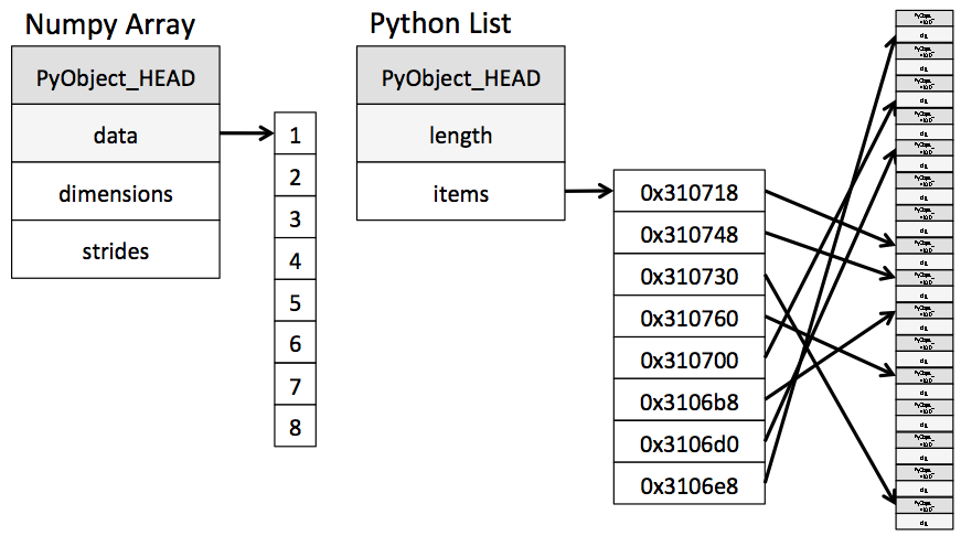
This is where NumPy arrays come into the picture. They require the contained data to be homogeneous (disregarding the “object” datatype), leading to a simpler structure of the underlying implementation: A NumPy array is an object with a pointer to a contiguous block of data in the memory.
NumPy forces the elements in its array to be homogeneous, by means of “upcasting”:
arr = np.array([1, 2, 3.14, 4])
arr  # upcasted to float, not "object", since it's much slower
array([1. , 2. , 3.14, 4. ])
This homogeneity and contiguity allows NumPy to use “vectorized” functions, which are simply functions that can iterate in C code over the array, as opposed to regular functions which have to use the Python iteration rules.
This means that while in essence the following two pieces of code are identical, the performance gain is due to the loop being done in C rather than in Python (this is the case in MATLAB as well):
%%timeit
python_array = list(range(1_000_000))
for item in python_array:
    item += 1
99.7 ms ± 1.34 ms per loop (mean ± std. dev. of 7 runs, 10 loops each)
%%timeit
numpy_array = np.arange(1_000_000)
numpy_array += 1  # inside, a C loop is adding 1 to each item.

# Two orders of magnitude improvement for a pretty small (1M elements) array.
# This is approximately the size of a 1024x1024 pixel image.
1.16 ms ± 7.44 µs per loop (mean ± std. dev. of 7 runs, 1000 loops each)
If you recall the first class, you’ll remember that we mentioned how Python code has to be transpiled into C code, which is then compiled to machine code. NumPy arrays take a “shortcut” here, are are quickly compiled to efficient C code without the Python overhead. When using vectorized NumPy operations, the loop Python does in the backstage is very similar to a loop that a C programmer would have written by hand.
Another small but significant benefit of NumPy arrays is smaller memory footprint:
from sys import getsizeof

python_array = list(range(1_000_000))
list_size = getsizeof(python_array) / 1e6  # in MB
print(f"Python list size (1M elements, MB): {list_size}")

numpy_array = np.arange(1_000_000, dtype=np.int32)
numpy_size = numpy_array.nbytes / 1e6
print(f"Numpy array size (1M elements, MB): {numpy_size}")
Python list size (1M elements, MB): 8.000056
Numpy array size (1M elements, MB): 4.0
Why do 1 million elements require 4MB?
Each element has to weigh 4 bytes, or 32 bits. This means that the np.arange() function generates by default int32 values.
Lower memory usage can help us pack larger array in the computer’s working memory (RAM), and it will also improve the performance of the underlying code.
Indexing and slicing
Indexing numpy arrays is very much what you’d expect it to be.
a = np.arange(10)
a[0], a[3], a[-2]  # Python indexing is always done with square brackets
(0, 3, 8)
The beautiful reverse slicing works here as well:
a[::-1]
array([9, 8, 7, 6, 5, 4, 3, 2, 1, 0])
arr_2d
array([[1, 2, 3],
       [4, 5, 6]])
arr_2d[0, 2] # first row, third column
3
arr_2d[0, :] # first row, all columns
array([1, 2, 3])
arr_2d[0]  # first item in the first dimension, and all of its corresponding elemets
# Similar to arr_2d[0, :]
array([1, 2, 3])
a[1::2]
array([1, 3, 5, 7, 9])
a[:2] # last index isn't included
array([0, 1])
View vs. Copy
In Python, slicing creates a view of an object, not a copy:
b = a[::2]
b
array([0, 2, 4, 6, 8])
b[0] = 100
b
array([100, 2, 4, 6, 8])
a # a is also changed!
array([100, 1, 2, 3, 4, 5, 6, 7, 8, 9])
Copying is done with copy():
a_copy = a[::-1].copy()
a_copy
array([ 9, 8, 7, 6, 5, 4, 3, 2, 1, 100])
a_copy[1] = 200
a_copy
array([ 9, 200, 7, 6, 5, 4, 3, 2, 1, 100])
a # unchanged
array([100, 1, 2, 3, 4, 5, 6, 7, 8, 9])
This behavior allows NumPy to save time and memory. It will usually go unnoticed during day-to-day use. Occasionally, however, it can result in ugly bugs which are hard to locate.
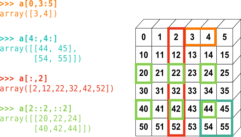
Let’s look at a summary of 2D indexing:
Aggregation
arr = np.random.random(1_000)
sum(arr)  # The native Python sum works on numpy arrays, but its use is discouraged in this context
500.6927534020991
sum() is a built-in Python function, capable of working on lists and other native Python data structures. NumPy has its own sum functions: You can either write np.sum(arr), or use arr.sum():
%timeit sum(arr)
%timeit np.sum(arr)
%timeit arr.sum()
100 µs ± 978 ns per loop (mean ± std. dev. of 7 runs, 10000 loops each)
5.19 µs ± 19 ns per loop (mean ± std. dev. of 7 runs, 100000 loops each)
3.25 µs ± 17.4 ns per loop (mean ± std. dev. of 7 runs, 100000 loops each)
Keep in mind that the built-in sum() and numpy’s np.sum() aren’t identical. np.sum() by default calculates the sum of all axes, returning a single number for multi-dimensional arrays.
In MATLAB, this behavior is replicated with sum(arr(:)).
Likewise, min() and max() also have two “competing” versions:
%timeit min(arr)  # Native Python
%timeit np.min(arr)
%timeit arr.min()
76.4 µs ± 130 ns per loop (mean ± std. dev. of 7 runs, 10000 loops each)
5.1 µs ± 20 ns per loop (mean ± std. dev. of 7 runs, 100000 loops each)
3.32 µs ± 13.5 ns per loop (mean ± std. dev. of 7 runs, 100000 loops each)
Calculating the min of an array will, again, result in a single number:
arr2 = np.random.random((4, 4, 4))
arr2.min()
0.010978859434496502
If you wish to calculate it across an axis, use the axis keyword:
arr2.min(axis=0)
array([[0.17597733, 0.07342398, 0.06232941, 0.11067078],
       [0.16992801, 0.24922993, 0.01381182, 0.2547518 ],
       [0.19839256, 0.22547658, 0.06554285, 0.48883579],
       [0.22017492, 0.69003167, 0.01097886, 0.13016616]])
2D output (axis number 0 was “dropped”)
arr2.max(axis=(0, 1))
array([0.9560919 , 0.95500034, 0.99231603, 0.94799179])
1D output (the two first axes were summed over)
Many other aggregation functions exist, including:
- np.var
- np.std
- np.argmin\argmax
- np.median
- ...
Most of them have an object-oriented version, i.e. arr.var(), and a procedural version, i.e. np.var(arr).
Fancy indexing
In NumPy, indexing an array with a different array is called “fancy” indexing. Perhaps confusingly, it creates a copy, not a view.
basic_array = np.arange(10)
basic_array
array([0, 1, 2, 3, 4, 5, 6, 7, 8, 9])
mask = (basic_array % 2 == 0)
mask
array([ True, False,  True, False,  True, False,  True, False,  True,
       False])
b = basic_array[mask]  # also basic_array[basic_array % 2 == 0]
b
array([0, 2, 4, 6, 8])
MATLAB veterans shouldn’t be surprised from this feature, but if you haven’t seen it before make sure to have a firm grasp on it, as it’s a very powerful technique.
b[:] = 999
print(f"basic array: {basic_array}")
print(f"b: {b}")
basic array: [0 1 2 3 4 5 6 7 8 9]
b: [999 999 999 999 999]
float_array = np.arange(start=0, stop=20, step=1.5)
float_array
array([ 0. ,  1.5,  3. ,  4.5,  6. ,  7.5,  9. , 10.5, 12. , 13.5, 15. ,
       16.5, 18. , 19.5])
float_array[[1, 2, 5, 5, 10]]  # copy, not a view. Meaning that the resulting array is a new
# instance of the original array, independent of it, in a different location in memory.
array([ 1.5, 3. , 7.5, 7.5, 15. ])
Counting the amount of values that fit our condition can be done as follows:
basic_array = np.arange(10)
count_nonzero_result = np.count_nonzero(basic_array % 2 == 0)
sum_result = np.sum(basic_array % 2 == 0)

print(f"np.count_nonzero result: {count_nonzero_result}")
print(f"np.sum result: {sum_result}")
# In the latter case, True is 1 and False is 0
np.count_nonzero result: 5
np.sum result: 5
If we wish to add more conditions in to the mix, we can use the &, |, ~, ^ operators (and, or, not, xor):
((basic_array % 2 == 1) & (basic_array != 3)).sum() # uneven values that are different from 3
4
Note that numpy uses the &, |, ~, ^ operators for element-by-element comparison, while the reserved and and or keywords evaluate the entire object:
np.sum((basic_array % 2 == 1) and (basic_array != 3)) # doesn't work, "and" isn't used this way here
---------------------------------------------------------------------------
ValueError                                Traceback (most recent call last)
<ipython-input-59-e462a6643cbd> in <module>
----> 1 np.sum((basic_array % 2 == 1) and (basic_array != 3))   # doesn't work, "and" isn't used this way here

ValueError: The truth value of an array with more than one element is ambiguous. Use a.any() or a.all()
Sorting
Again we face a condition in which Python has its own sort functions, but numpy’s np.sort() are much better suited for arrays. We can either sort in-place, or have a new object back:
# Return a new object:
arr = np.array([ 3, 4, 1, 8, 10, 2, 4])
print(np.sort(arr))

# Sort in-place:
arr.sort()
print(arr)
[ 1  2  3  4  4  8 10]
[ 1  2  3  4  4  8 10]
The default implementation is a quicksort but other sorting algorithms can be found as well.
# np.argsort will return the indices of the sorted array:
arr = np.array([ 3, 4, 1, 8, 10, 2, 4])
print("Sorted indices: {}".format(np.argsort(arr)))

# Usage is as follows:
arr[np.argsort(arr)]
Sorted indices: [2 5 0 1 6 3 4]
array([ 1, 2, 3, 4, 4, 8, 10])
Concatenation
Concatenation (and splitting) in numpy works as follows:
x = np.array([1, 2, 3])
y = np.array([3, 2, 1])
np.concatenate([x, y])  # concatenates along the first axis
array([1, 2, 3, 3, 2, 1])
# Concatenate more than two arrays
z = [99, 99, 99]
np.concatenate([x, y, z])  # notice how the function argument is an iterable!
array([ 1, 2, 3, 3, 2, 1, 99, 99, 99])
# 2D - along the last axis
twod_1 = np.array([[0, 1, 2],
                   [3, 4, 5]])
twod_2 = np.array([[6, 7, 8],
                   [9, 10, 11]])
np.concatenate((twod_1, twod_2), axis=-1)
array([[ 0,  1,  2,  6,  7,  8],
       [ 3,  4,  5,  9, 10, 11]])
np.vstack() and np.hstack() are also an option:
sim1 = np.array([0, 1, 2])
sim2 = np.array([[30, 40, 50],
                 [60, 70, 80]])
np.vstack((sim1, sim2))
array([[ 0,  1,  2],
       [30, 40, 50],
       [60, 70, 80]])
Splitting up arrays is also quite easy:
arr = np.arange(16).reshape((4, 4))  # see the tuple? Shapes of arrays always come in tuples
arr
array([[ 0,  1,  2,  3],
       [ 4,  5,  6,  7],
       [ 8,  9, 10, 11],
       [12, 13, 14, 15]])
upper, lower = np.split(arr, [3])  # splits at the fourth line (of the first axis, by default)
print(upper)
print('---')
print(lower)
[[ 0  1  2  3]
 [ 4  5  6  7]
 [ 8  9 10 11]]
---
[[12 13 14 15]]
Exercise
a. Familiarization:
Create two random 3D arrays, at least 3x3x3 in size. The first should have random integers between 0 and 100, while the second should contain floating points numbers drawn from the normal distribution, with mean -1 and standard deviation of 2
What are the default datatypes of integer and floating-point arrays in numpy?
Center the distribution of the first integer array around 0, with values between -1 and 1.
Caclulate their mean, standard deviation along the last axis, and sum along the second axis. Remember that arrays are, like everything in Python, objects.
b. Iteration over an array:
Find and return the indices of the two random arrays only where both elements comply with -0.5 <= X <= 0.5. Do so in at least two distinct ways. These can include elementwise iteration, masked-arrays, and more.
Time the execution of the script using the IPython %%timeit magic if you have this tool near at hand.
c. Broadcasting:
Create a vector with length 100, filled with ones, and a 2D zero-filled array with its last dimension with size of 100.
Using
np.tile, add the vector and the array.Did you have to use
np.tilein this case? What feature of numpy allows this?What happens to the non-tiled addition when the first dimension of the matrix is 100? Why?
Bonus: How can one add the matrix (in its new shape) and vector without np.tile()?
Exercise solutions below…
# a
# 1
low = 0
high = 100
arr1 = np.random.randint(low=low, high=high, size=(10, 10, 10))  # dtype is np.int32
arr2 = np.random.randn(10, 10, 10) * 2 - 1  # dtype is np.float64

# 2
middle = (high - low) / 2
arr1 = (arr1 - middle) / middle

# 3
print("arr1 (integers) stats:")
print(f"Mean: {arr1.mean()},\nSTD: {arr1.std(axis=-1)},\nSum: {arr1.sum(axis=1)}")
print("arr2 (normal distribution) stats:")
print(f"Mean: {arr2.mean()},\nSTD: {arr2.std(axis=-1)},\nSum: {arr2.sum(axis=1)}")
arr1 (integers) stats:
Mean: -0.003299999999999993,
STD: [[0.61413028 0.63496772 0.579341   0.45338284 0.59375416 0.55993214
  0.51947666 0.49316934 0.71838987 0.56886202]
 [0.51645329 0.43699428 0.64967684 0.50187249 0.60078615 0.4678846
  0.63074876 0.58931825 0.51452502 0.38107217]
 [0.57787542 0.46953594 0.57229713 0.64358061 0.62834704 0.56277882
  0.60306219 0.60471481 0.48009999 0.58577811]
 [0.52890831 0.44567253 0.4455289  0.68385963 0.53222552 0.64355575
  0.46972758 0.59821067 0.65124189 0.418     ]
 [0.4765543  0.55117692 0.50059565 0.56475127 0.5747382  0.46067776
  0.56067459 0.67830377 0.43528841 0.61065211]
 [0.63437844 0.62091545 0.43064603 0.55252511 0.63226893 0.55666507
  0.60571941 0.62086714 0.46270941 0.61284908]
 [0.64875573 0.61807767 0.50119856 0.38616577 0.6899971  0.51975379
  0.62476876 0.50255348 0.62355112 0.5937811 ]
 [0.67498148 0.53414979 0.42307919 0.54124301 0.57255917 0.42455153
  0.5869787  0.61057678 0.42227953 0.4565961 ]
 [0.55015998 0.55504955 0.52557017 0.52084547 0.46825634 0.63206329
  0.64696522 0.35293625 0.64850906 0.53126641]
 [0.39809547 0.41503735 0.64527823 0.52391221 0.58352378 0.56970519
  0.61299266 0.68860439 0.37049157 0.46916522]],
Sum: [[ 0.6   0.76 -1.46  0.78 -0.52  0.28 -0.44  2.38  1.5  -0.56]
 [ 1.52  1.28 -0.22 -2.6  -0.72  1.3   2.28 -1.32 -2.5  -0.92]
 [-3.3   0.24  0.06  5.7  -0.6  -1.18  2.46 -1.46  1.22  4.6 ]
 [-0.2  -0.62 -0.18 -1.88  0.26  0.9  -1.34 -1.52 -1.12  0.1 ]
 [-1.34 -0.48  3.54  0.02 -1.74 -3.28 -1.6   0.04 -0.44  0.18]
 [-0.2  -0.82  2.48 -0.08  1.12  1.76  0.78  0.82 -0.7   1.52]
 [ 0.68 -1.2   1.24  0.96  1.98 -1.56 -0.42  1.42 -1.7   2.18]
 [-2.08 -0.52 -0.86  2.66  0.3  -0.16 -2.08  1.12 -1.56 -3.06]
 [-1.48  0.44 -3.8   0.78 -0.46 -2.34 -1.02 -3.36  0.48  3.78]
 [ 1.94 -2.82  0.74  0.48 -1.92 -0.74  2.96  2.14 -3.02  1.44]]
arr2 (normal distribution) stats:
Mean: -1.0660585666527882,
STD: [[2.31544927 1.77718883 2.10931233 2.07086989 2.01507156 1.79707925
  2.00243897 2.51897746 1.44454278 1.8063456 ]
 [1.80419386 2.25656497 2.73481099 2.03735892 1.32516534 2.2981038
  2.03615381 1.15112356 1.87981976 1.3265946 ]
 [1.48642687 1.24976502 1.3302147  2.19646823 2.06313093 2.07408853
  1.8430677  1.29160461 2.81555997 2.57809888]
 [2.27342767 1.70774397 1.5208181  1.22537661 1.5237457  2.93904086
  1.71740143 1.83819469 1.99706647 1.74497977]
 [2.22282999 2.47349249 2.14261593 2.38518479 1.80188576 1.39155671
  2.08749412 1.92163688 2.46220221 1.9627998 ]
 [2.05119588 2.59213132 1.88875396 1.59855884 1.28506862 1.32263345
  2.04679749 1.71558551 1.28251315 1.31145428]
 [1.49929653 1.42529623 1.65581838 1.59207708 1.29527799 2.95324976
  1.97477342 1.25380272 1.58895471 2.29024052]
 [1.93085593 2.28185223 1.92493486 2.77577824 1.97947008 2.24246452
  1.26531158 2.2728571  1.62609895 1.49026967]
 [1.63946897 2.72394821 1.41114442 2.02096689 1.69689438 2.28502105
  1.42469594 1.92400498 1.78349657 1.6531562 ]
 [1.81440544 1.03221459 2.55311532 1.48723677 1.91455406 2.4527401
  2.04005407 1.94469084 2.31325275 1.86772573]],
Sum: [[ -9.40027742  -3.36161039 -14.91969082 -11.32231488  -2.66534013
  -12.29594213  -5.95680511 -10.07323285   1.40987566 -19.29167811]
 [-18.35125791  -7.28350574  -8.78439871 -19.30469964 -11.16513675
   -6.65224395  -3.29751313  -2.25131205  -3.15043635 -13.52352302]
 [-16.47789896 -11.05044588  -7.70596747 -14.19820125 -15.96462027
  -16.18389494  -7.25006129  -9.01446973 -17.41697305  -9.2034521 ]
 [-12.2346333  -20.45296706 -18.82857133 -19.96934899 -16.01228039
   -1.50829099  -3.27949371 -10.17283648 -15.75495358  -5.39211986]
 [-10.65956725   0.60603493 -12.82321353  -8.28373165 -12.28355216
  -24.03574812 -12.32377722  -8.02187555 -12.28440639 -15.44851808]
 [-10.71145495   3.07996488 -14.06204908  -4.87529983  -7.96215363
    3.14582087 -20.35718368   1.69559473 -11.49107834 -17.32151182]
 [-11.99843766 -18.4382233  -10.49386551 -16.48637583  -9.33345803
  -10.51880216  -6.93463917 -20.79650028  -5.0352572   -8.4557133 ]
 [-10.61432866 -10.42964346  -8.77462003 -19.25280973  -9.14209326
   -0.35083695  -4.91678299  -3.36467552 -20.91942723 -10.16639792]
 [-11.26389202 -13.88405571  -5.84920013  -7.21240978 -16.25834344
  -18.16492379  -9.19961895 -19.14322753  -6.35901697  -7.16871857]
 [ -4.25951886  -0.65254982 -19.36146819 -16.28293654 -18.41323254
   -6.71099642  -6.69260484 -14.02991628 -12.87765991 -11.72115824]]
%%timeit
# b
# 1 - elementwise
result = []
for idx, (item1, item2) in enumerate(zip(arr1.flat, arr2.flat)):
    if (-0.5 <= item1 <= 0.5) and (-0.5 <= item2 <= 0.5):
        result.append(idx)
result
409 µs ± 1.15 µs per loop (mean ± std. dev. of 7 runs, 1000 loops each)
%%timeit
# b
# 2 - masked arrays createed by np.ravel(), np.where()
mask1 = ((-0.5 <= arr1.ravel()) & (arr1.ravel() <= 0.5))
mask2 = ((-0.5 <= arr2.ravel()) & (arr2.ravel() <= 0.5))
both_positive = np.logical_and(mask1, mask2)
result = np.where(both_positive)
result
10.5 µs ± 12.5 ns per loop (mean ± std. dev. of 7 runs, 100000 loops each)
As you can tell, the second solution is far more efficient than the first, and after a few read code blocks, the syntax presented there can be at least as clear as the one in the first solution.
# c
# 1
vec = np.ones(100)
mat = np.zeros((10, 100))

# 2
tiled_vec = np.tile(vec, (10, 1))  # transpose is necessary
ans_tiled = mat + tiled_vec

# 3
ans_simple = mat + vec  # It's called array broadcasting

# 4
mat_transposed = mat.T
print(mat_transposed.shape)
# ans_trans = mat_transposed + vec  # fails because broadcasting is done over the last dimension

# 5 - np.newaxis is the answer - very perfomant
ans_newaxis = mat_transposed + vec[:, np.newaxis]
(100, 10)