Class 7: Advanced pandas#
Currently, pandas’ Series and DataFrame might seem to us as no more than tables with complicated indexing methods. In this lesson, we will learn more about what makes pandas so powerful and how we can use it to write efficient and readable code.
Note
Some of the features described below only work with pandas >= 1.0.0. Make sure you have the latest pandas installation when running this notebook. To check the version of your pandas (or any other package), import it and print its __version__ attribute:
>>> import pandas as pd
>>> print(pd.__version__)
'2.2.3'
Missing Data#

The last question in the previous class pointed us to working with missing data. But how and why do missing data occur?
One option is pandas’ index alignment, the property that makes sure that each value will have the same index throughout the entire computation process.
import pandas as pd
import numpy as np


A = pd.Series([2, 4, 6], index=[0, 1, 2])
B = pd.Series([1, 3, 5], index=[1, 2, 3])
A + B
0    NaN
1    5.0
2    9.0
3    NaN
dtype: float64
The NaNs we have are what we call missing data, and this is how they are represented in pandas. We’ll discuss that in more detail in a few moments.
The same thing occurs with DataFrames:
A = pd.DataFrame(np.random.randint(0, 20, (2, 2)),
                 columns=list('AB'))
A
| A | B | |
|---|---|---|
| 0 | 9 | 11 |
| 1 | 11 | 9 |
B = pd.DataFrame(np.random.randint(0, 10, (3, 3)),
                 columns=list('BAC'))
B
| B | A | C | |
|---|---|---|---|
| 0 | 7 | 8 | 7 |
| 1 | 6 | 1 | 5 |
| 2 | 3 | 1 | 1 |
new = A + B
print(new)
print(f"\nReturned dtypes:\n{new.dtypes}")
      A     B   C
0  17.0  18.0 NaN
1  12.0  15.0 NaN
2   NaN   NaN NaN

Returned dtypes:
A    float64
B    float64
C    float64
dtype: object
Note
Note how new.dtypes itself returns a Series of dtypes, with it’s own object dtype.
The dataframe’s shape is the shape of the larger dataframe, and the “extra” row (index 2) was filled with NaNs. Since we have NaNs, the data type of the column is implicitly converted to a floating point type. To have integer dataframes with NaNs, we have to explicitly say we want them available. More on that later.
Another way to introduce missing data is through reindexing. If we “resample” our data we can achieve the following:
df = pd.DataFrame(np.random.randn(5, 3), index=['a', 'c', 'e', 'f', 'h'],
                  columns=['one', 'two', 'three'])
df
| one | two | three | |
|---|---|---|---|
| a | -0.738739 | 1.639344 | 0.633690 |
| c | -1.451243 | -1.126693 | -1.093036 |
| e | -0.343553 | -0.530344 | 1.038596 |
| f | 0.135088 | 0.393802 | 0.368759 |
| h | 0.792737 | 1.208998 | 1.494570 |
df2 = df.reindex(['a', 'b', 'c', 'd', 'e', 'f', 'g', 'h'])
df2
| one | two | three | |
|---|---|---|---|
| a | -0.738739 | 1.639344 | 0.633690 |
| b | NaN | NaN | NaN |
| c | -1.451243 | -1.126693 | -1.093036 |
| d | NaN | NaN | NaN |
| e | -0.343553 | -0.530344 | 1.038596 |
| f | 0.135088 | 0.393802 | 0.368759 |
| g | NaN | NaN | NaN |
| h | 0.792737 | 1.208998 | 1.494570 |
But what is NaN? Is it the same as None? To better answer the former, let’s first have a closer look at the latter.
The None object#
None is the standard null value in Python, and is used extensively in normal usage of the language. For example, functions that don’t have a return statement, implicitly return None. While None can be used as a missing data type, it’s probably not the best choice.
vals1 = np.array([1, None, 3, 4])
vals1
array([1, None, 3, 4], dtype=object)
The dtype is object, because the best common type of ints and a None is a Python object. This slows down computation time on these arrays:
for dtype in ['object', 'int']:
    print("dtype =", dtype)
    %timeit np.arange(1E6, dtype=dtype).sum()
    print()
dtype = object
40.6 ms ± 1.76 ms per loop (mean ± std. dev. of 7 runs, 10 loops each)

dtype = int
343 μs ± 10.7 μs per loop (mean ± std. dev. of 7 runs, 1,000 loops each)
If you recall from a couple of lessons ago, the performance of object arrays is very similar to that of standard lists (generally speaking, the two data structures are effectively identical).
Another thing we can’t do is aggregation:
vals1.sum()
---------------------------------------------------------------------------
TypeError                                 Traceback (most recent call last)
Cell In[9], line 1
----> 1 vals1.sum()

File ~/Projects/courses/python_for_neuroscientists/textbook-public/venv/lib/python3.11/site-packages/numpy/_core/_methods.py:53, in _sum(a, axis, dtype, out, keepdims, initial, where)
     51 def _sum(a, axis=None, dtype=None, out=None, keepdims=False,
     52          initial=_NoValue, where=True):
---> 53     return umr_sum(a, axis, dtype, out, keepdims, initial, where)

TypeError: unsupported operand type(s) for +: 'int' and 'NoneType'
The NaN value#
NaN is a special floating-point value recognized by all programming languages that conform to the IEEE standard (which means most of them). As we mentioned before, it forces the entire array to have a floating point type:
vals2 = np.array([1, np.nan, 3, 4])
vals2.dtype
dtype('float64')
Creating floating point arrays is very fast, so performance isn’t hindered. NaN is sometimes described as a “data virus”, since it infects objects it touches:
1 + np.nan
nan
0 * np.nan
nan
vals2.sum(), vals2.min(), vals2.max()
(np.float64(nan), np.float64(nan), np.float64(nan))
np.nan == np.nan
False
Numpy has nan-aware counterparts to many of its aggregation functions, which can work with NaNs correctly. They usually have the same name as their non-NaN sibling, but with the “nan” prefix:
print(np.nansum(vals2))
print(np.nanmean(vals2))
8.0
2.6666666666666665
However, pandas objects account for NaNs in their calculations, as we’ll soon see.
Pandas can handle both NaN and None interchangeably:
ser = pd.Series([1, np.nan, 2, None])
ser
0    1.0
1    NaN
2    2.0
3    NaN
dtype: float64
The NaT value#
When dealing with datetime values or indices, the missing value is represented as NaT, or not-a-time:

df['timestamp'] = pd.Timestamp('20180101')
df
| one | two | three | timestamp | |
|---|---|---|---|---|
| a | -0.738739 | 1.639344 | 0.633690 | 2018-01-01 |
| c | -1.451243 | -1.126693 | -1.093036 | 2018-01-01 |
| e | -0.343553 | -0.530344 | 1.038596 | 2018-01-01 |
| f | 0.135088 | 0.393802 | 0.368759 | 2018-01-01 |
| h | 0.792737 | 1.208998 | 1.494570 | 2018-01-01 |
df2 = df.reindex(['a', 'b', 'c', 'd', 'e', 'f', 'g', 'h'])
df2
| one | two | three | timestamp | |
|---|---|---|---|---|
| a | -0.738739 | 1.639344 | 0.633690 | 2018-01-01 |
| b | NaN | NaN | NaN | NaT |
| c | -1.451243 | -1.126693 | -1.093036 | 2018-01-01 |
| d | NaN | NaN | NaN | NaT |
| e | -0.343553 | -0.530344 | 1.038596 | 2018-01-01 |
| f | 0.135088 | 0.393802 | 0.368759 | 2018-01-01 |
| g | NaN | NaN | NaN | NaT |
| h | 0.792737 | 1.208998 | 1.494570 | 2018-01-01 |
Operations and calculations with missing data#
a = pd.DataFrame(np.random.random((5, 2)), columns=['one', 'two'])
a.iloc[1, 1] = np.nan
a
| one | two | |
|---|---|---|
| 0 | 0.381413 | 0.994560 |
| 1 | 0.831090 | NaN |
| 2 | 0.422959 | 0.226737 |
| 3 | 0.335573 | 0.208971 |
| 4 | 0.051523 | 0.611757 |
b = pd.DataFrame(np.random.random((6, 3)), columns=['one', 'two', 'three'])
b.iloc[2, 2] = np.nan
b
| one | two | three | |
|---|---|---|---|
| 0 | 0.145631 | 0.043131 | 0.724304 |
| 1 | 0.843106 | 0.705622 | 0.077469 |
| 2 | 0.422559 | 0.301640 | NaN |
| 3 | 0.018374 | 0.622743 | 0.332941 |
| 4 | 0.504732 | 0.970574 | 0.045283 |
| 5 | 0.502859 | 0.940474 | 0.628992 |
a + b
| one | three | two | |
|---|---|---|---|
| 0 | 0.527044 | NaN | 1.037691 |
| 1 | 1.674196 | NaN | NaN |
| 2 | 0.845518 | NaN | 0.528377 |
| 3 | 0.353947 | NaN | 0.831714 |
| 4 | 0.556255 | NaN | 1.582331 |
| 5 | NaN | NaN | NaN |
As we see, missing values propagate naturally through these arithmetic operations. Statistics also works:
(a + b).describe()
# Summation - NaNs are zero.
# If everything is NaN - the result is NaN as well.
# pandas' cumsum and cumprod ignore NaNs but preserve them in the resulting arrays.
| one | three | two | |
|---|---|---|---|
| count | 5.000000 | 0.0 | 4.000000 |
| mean | 0.791392 | NaN | 0.995028 |
| std | 0.524118 | NaN | 0.443914 |
| min | 0.353947 | NaN | 0.528377 |
| 25% | 0.527044 | NaN | 0.755880 |
| 50% | 0.556255 | NaN | 0.934703 |
| 75% | 0.845518 | NaN | 1.173851 |
| max | 1.674196 | NaN | 1.582331 |
We can also receive a boolean mask of the NaNs in a dataframe:
mask = (a + b).isnull()  # also isna(), and the opposite .notnull()
mask
| one | three | two | |
|---|---|---|---|
| 0 | False | True | False |
| 1 | False | True | True |
| 2 | False | True | False |
| 3 | False | True | False |
| 4 | False | True | False |
| 5 | True | True | True |
Filling missing values#
The simplest option is to use the fillna method:
summed = a + b
summed.iloc[4, 0] = np.nan
summed
| one | three | two | |
|---|---|---|---|
| 0 | 0.527044 | NaN | 1.037691 |
| 1 | 1.674196 | NaN | NaN |
| 2 | 0.845518 | NaN | 0.528377 |
| 3 | 0.353947 | NaN | 0.831714 |
| 4 | NaN | NaN | 1.582331 |
| 5 | NaN | NaN | NaN |
summed.fillna(0)
| one | three | two | |
|---|---|---|---|
| 0 | 0.527044 | 0.0 | 1.037691 |
| 1 | 1.674196 | 0.0 | 0.000000 |
| 2 | 0.845518 | 0.0 | 0.528377 |
| 3 | 0.353947 | 0.0 | 0.831714 |
| 4 | 0.000000 | 0.0 | 1.582331 |
| 5 | 0.000000 | 0.0 | 0.000000 |
summed.fillna('missing') # changed dtype to "object"
| one | three | two | |
|---|---|---|---|
| 0 | 0.527044 | missing | 1.037691 |
| 1 | 1.674196 | missing | missing |
| 2 | 0.845518 | missing | 0.528377 |
| 3 | 0.353947 | missing | 0.831714 |
| 4 | missing | missing | 1.582331 |
| 5 | missing | missing | missing |
summed.ffill()  # The NaN column remained the same, but values were propagated forward
# We can also use the "backfill" method to fill in values to the back
| one | three | two | |
|---|---|---|---|
| 0 | 0.527044 | NaN | 1.037691 |
| 1 | 1.674196 | NaN | 1.037691 |
| 2 | 0.845518 | NaN | 0.528377 |
| 3 | 0.353947 | NaN | 0.831714 |
| 4 | 0.353947 | NaN | 1.582331 |
| 5 | 0.353947 | NaN | 1.582331 |
summed.ffill(limit=1) # No more than one padded NaN in a row
| one | three | two | |
|---|---|---|---|
| 0 | 0.527044 | NaN | 1.037691 |
| 1 | 1.674196 | NaN | 1.037691 |
| 2 | 0.845518 | NaN | 0.528377 |
| 3 | 0.353947 | NaN | 0.831714 |
| 4 | 0.353947 | NaN | 1.582331 |
| 5 | NaN | NaN | 1.582331 |
summed.fillna(summed.mean()) # each column received its respective mean. The NaN column is untouched.
| one | three | two | |
|---|---|---|---|
| 0 | 0.527044 | NaN | 1.037691 |
| 1 | 1.674196 | NaN | 0.995028 |
| 2 | 0.845518 | NaN | 0.528377 |
| 3 | 0.353947 | NaN | 0.831714 |
| 4 | 0.850176 | NaN | 1.582331 |
| 5 | 0.850176 | NaN | 0.995028 |
Dropping missing values#
We’ve already seen in the short exercise the dropna method, that allows us to drop missing values:
summed
| one | three | two | |
|---|---|---|---|
| 0 | 0.527044 | NaN | 1.037691 |
| 1 | 1.674196 | NaN | NaN |
| 2 | 0.845518 | NaN | 0.528377 |
| 3 | 0.353947 | NaN | 0.831714 |
| 4 | NaN | NaN | 1.582331 |
| 5 | NaN | NaN | NaN |
filled = summed.fillna(summed.mean())
filled
| one | three | two | |
|---|---|---|---|
| 0 | 0.527044 | NaN | 1.037691 |
| 1 | 1.674196 | NaN | 0.995028 |
| 2 | 0.845518 | NaN | 0.528377 |
| 3 | 0.353947 | NaN | 0.831714 |
| 4 | 0.850176 | NaN | 1.582331 |
| 5 | 0.850176 | NaN | 0.995028 |
filled.dropna(axis=1) # each column containing NaN is dropped
| one | two | |
|---|---|---|
| 0 | 0.527044 | 1.037691 |
| 1 | 1.674196 | 0.995028 |
| 2 | 0.845518 | 0.528377 |
| 3 | 0.353947 | 0.831714 |
| 4 | 0.850176 | 1.582331 |
| 5 | 0.850176 | 0.995028 |
filled.dropna(axis=0) # each row containing a NaN is dropped
| one | three | two |
|---|
Interpolation#
The last way to to fill in missing values is through interpolation.
The default interpolation methods perform linear interpolation on the data, based on its ordinal index:
summed
| one | three | two | |
|---|---|---|---|
| 0 | 0.527044 | NaN | 1.037691 |
| 1 | 1.674196 | NaN | NaN |
| 2 | 0.845518 | NaN | 0.528377 |
| 3 | 0.353947 | NaN | 0.831714 |
| 4 | NaN | NaN | 1.582331 |
| 5 | NaN | NaN | NaN |
summed.interpolate() # notice all the details in the interpolation of the three columns
| one | three | two | |
|---|---|---|---|
| 0 | 0.527044 | NaN | 1.037691 |
| 1 | 1.674196 | NaN | 0.783034 |
| 2 | 0.845518 | NaN | 0.528377 |
| 3 | 0.353947 | NaN | 0.831714 |
| 4 | 0.353947 | NaN | 1.582331 |
| 5 | 0.353947 | NaN | 1.582331 |
We can also interpolate with the actual index values in mind:
# Create "missing" index
timeindex = pd.Series(['1/1/2018', '1/4/2018', '1/5/2018', '1/7/2018', '1/8/2018'])
timeindex = pd.to_datetime(timeindex)
data_to_interp = [1, np.nan, 5, np.nan, 8]
df_to_interp = pd.DataFrame(data_to_interp, index=timeindex)
df_to_interp
| 0 | |
|---|---|
| 2018-01-01 | 1.0 |
| 2018-01-04 | NaN |
| 2018-01-05 | 5.0 |
| 2018-01-07 | NaN |
| 2018-01-08 | 8.0 |
df_to_interp.interpolate() # the index values aren't taken into account
| 0 | |
|---|---|
| 2018-01-01 | 1.0 |
| 2018-01-04 | 3.0 |
| 2018-01-05 | 5.0 |
| 2018-01-07 | 6.5 |
| 2018-01-08 | 8.0 |
df_to_interp.interpolate(method='index') # notice how the data obtains the "right" values
| 0 | |
|---|---|
| 2018-01-01 | 1.0 |
| 2018-01-04 | 4.0 |
| 2018-01-05 | 5.0 |
| 2018-01-07 | 7.0 |
| 2018-01-08 | 8.0 |
Pandas has many other interpolation methods, based on SciPy’s.
df_inter_2 = pd.DataFrame({'A': [1, 2.1, np.nan, 4.7, 5.6, 6.8],
                           'B': [.25, np.nan, np.nan, 4, 12.2, 14.4]})
df_inter_2
| A | B | |
|---|---|---|
| 0 | 1.0 | 0.25 |
| 1 | 2.1 | NaN |
| 2 | NaN | NaN |
| 3 | 4.7 | 4.00 |
| 4 | 5.6 | 12.20 |
| 5 | 6.8 | 14.40 |
df_inter_2.interpolate(method='polynomial', order=2)
| A | B | |
|---|---|---|
| 0 | 1.000000 | 0.250000 |
| 1 | 2.100000 | -2.703846 |
| 2 | 3.451351 | -1.453846 |
| 3 | 4.700000 | 4.000000 |
| 4 | 5.600000 | 12.200000 |
| 5 | 6.800000 | 14.400000 |
Missing Values in Non-Float Columns#
Starting from pandas v1.0.0 pandas gained support for NaN values in non-float columns. This feature is a bit experimental currently, so the default behavior still converts integers to floats for example, but the support is there if you know where to look. By default:
nanint = pd.Series([1, 2, np.nan, 4])
nanint  # the result has a dtype of float64 even though all numbers are integers.
0    1.0
1    2.0
2    NaN
3    4.0
dtype: float64
We can try to force pandas’ hand here, but it won’t work:
nanint = pd.Series([1, 2, np.nan, 4], dtype="int32")
---------------------------------------------------------------------------
ValueError                                Traceback (most recent call last)
Cell In[46], line 1
----> 1 nanint = pd.Series([1, 2, np.nan, 4], dtype="int32")

File ~/Projects/courses/python_for_neuroscientists/textbook-public/venv/lib/python3.11/site-packages/pandas/core/series.py:584, in Series.__init__(self, data, index, dtype, name, copy, fastpath)
    582         data = data.copy()
    583 else:
--> 584     data = sanitize_array(data, index, dtype, copy)
    586     manager = _get_option("mode.data_manager", silent=True)
    587     if manager == "block":

File ~/Projects/courses/python_for_neuroscientists/textbook-public/venv/lib/python3.11/site-packages/pandas/core/construction.py:651, in sanitize_array(data, index, dtype, copy, allow_2d)
    648     subarr = np.array([], dtype=np.float64)
    650 elif dtype is not None:
--> 651     subarr = _try_cast(data, dtype, copy)
    653 else:
    654     subarr = maybe_convert_platform(data)

File ~/Projects/courses/python_for_neuroscientists/textbook-public/venv/lib/python3.11/site-packages/pandas/core/construction.py:818, in _try_cast(arr, dtype, copy)
    813 # GH#15832: Check if we are requesting a numeric dtype and
    814 # that we can convert the data to the requested dtype.
    815 elif dtype.kind in "iu":
    816     # this will raise if we have e.g. floats
--> 818     subarr = maybe_cast_to_integer_array(arr, dtype)
    819 elif not copy:
    820     subarr = np.asarray(arr, dtype=dtype)

File ~/Projects/courses/python_for_neuroscientists/textbook-public/venv/lib/python3.11/site-packages/pandas/core/dtypes/cast.py:1654, in maybe_cast_to_integer_array(arr, dtype)
   1646     with warnings.catch_warnings():
   1647         # We already disallow dtype=uint w/ negative numbers
   1648         # (test_constructor_coercion_signed_to_unsigned) so safe to ignore.
   1649         warnings.filterwarnings(
   1650             "ignore",
   1651             "NumPy will stop allowing conversion of out-of-bound Python int",
   1652             DeprecationWarning,
   1653         )
-> 1654         casted = np.asarray(arr, dtype=dtype)
   1655 else:
   1656     with warnings.catch_warnings():

ValueError: cannot convert float NaN to integer
To our rescue comes the new pd.Int32Dtype:
nanint = pd.Series([1, 2, np.nan, 4], dtype="Int32")
nanint
0       1
1       2
2    <NA>
3       4
dtype: Int32
It worked! We have a series with integers and a missing value! Notice the changes we had to made:
The
NaNis<NA>now. It’s actually a new type ofNaNcalledpd.NA.The data type had to be mentioned explictly, meaning that the conversion will work only if we know in advance that we’ll have NA values.
The data type is
Int32. It’s CamelCase and it’s actually a class underneath. Standard datatypes are lowercase.
Caveats aside, this is definitely useful for scientists who sometimes have integer values and do not want to convert them to float to supports NAs.
Exercise: Missing Data
Create a vector of 10000 measurements from a 10-cycle sinus wave. Remember that a single period of sine starts at 0 and ends at 2\(\pi\), so 10 periods span between 0 and 20\(\pi\).
Solution
n_cycles = 10
n_samples = 10000
amplitude = 3
phase = np.pi / 4
end = 2 * np.pi * n_cycles
x = np.linspace(0, end, num=n_samples)
y = amplitude * np.sin(x + phase)
Using
np.random.choice(replace=False)sample 100 points from the wave and place them in a Series.
Solution
chosen_idx = np.random.choice(n_samples, size=100, replace=False)
data = pd.DataFrame(np.nan, index=x, columns=['raw'])
data.iloc[chosen_idx, 0] = y[chosen_idx]
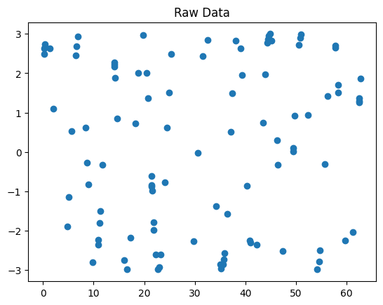
Plot the chosen points.
Solution
fig1, ax1 = plt.subplots()
ax1.set_title('Raw data pre-interpolation')
data.raw.plot(marker='o', ax=ax1)
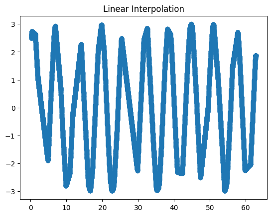
Interpolate the points using linear interpolation and plot them on a different graph.
Solution
data['lin_inter'] = data.raw.interpolate(method='index')
fig2, ax2 = plt.subplots()
ax2.set_title('Linear interpolation')
data.lin_inter.plot(marker='o', ax=ax2)
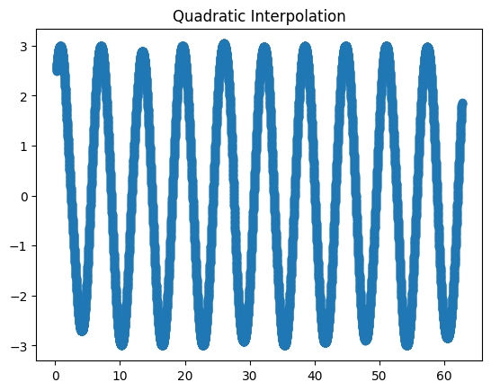
Interpolate the points using quadratic interpolation and plot them on a different graph.
Solution
data['quad_inter'] = data.raw.interpolate(method='quadratic')
fig3, ax3 = plt.subplots()
ax3.set_title('Quadratic interpolation')
data.quad_inter.plot(marker='o', ax=ax3)
Categorical Data#
So far, we’ve used examples with quantitative data. Let’s now have a look at categorical data, i.e. data can only have one of a specific set, or categories, of values. For example, if we have a column which marks the weekday, then it can obviously only be one of seven options. Same for boolean data, colors, and other examples. These data columns should be marked as “categorical” to reduce memory consumption and improve performance. It also tells the code readers more about the nature of that data column.
The easiest way to create a categorical variable is to declare it as such, or to convert as existing column to a categorical data type:
s = pd.Series(["a", "b", "c", "a"], dtype="category")
s
0    a
1    b
2    c
3    a
dtype: category
Categories (3, object): ['a', 'b', 'c']
df = pd.DataFrame({"A": ["a", "b", "c", "a"]})
df["B"] = df["A"].astype("category")
print(f"DataFrame:\n{df}")
print(f"\nData types:\n{df.dtypes}")
DataFrame:
   A  B
0  a  a
1  b  b
2  c  c
3  a  a

Data types:
A      object
B    category
dtype: object
We can also force order between our categories, or force specific categories on our data, using the special CategoricalDtype (which we won’t show).
As we said, memory usage is reduced when working with categorical data:
df_obj = pd.DataFrame({'a': np.random.random(10_000), 'b': ['a'] * 10_000})
df_obj
| a | b | |
|---|---|---|
| 0 | 0.955672 | a |
| 1 | 0.971781 | a |
| 2 | 0.772453 | a |
| 3 | 0.436727 | a |
| 4 | 0.515644 | a |
| ... | ... | ... |
| 9995 | 0.958149 | a |
| 9996 | 0.494567 | a |
| 9997 | 0.022768 | a |
| 9998 | 0.091958 | a |
| 9999 | 0.552508 | a |
10000 rows × 2 columns
df_cat = pd.DataFrame({'a': df_obj['a'], 'b': df_obj['b'].astype('category')})
df_cat
| a | b | |
|---|---|---|
| 0 | 0.955672 | a |
| 1 | 0.971781 | a |
| 2 | 0.772453 | a |
| 3 | 0.436727 | a |
| 4 | 0.515644 | a |
| ... | ... | ... |
| 9995 | 0.958149 | a |
| 9996 | 0.494567 | a |
| 9997 | 0.022768 | a |
| 9998 | 0.091958 | a |
| 9999 | 0.552508 | a |
10000 rows × 2 columns
df_obj.memory_usage()
Index      132
a        80000
b        80000
dtype: int64
df_cat.memory_usage()
Index      132
a        80000
b        10116
dtype: int64
A factor of 8 in memory reduction.
Hierarchical Indexing#
Last time we mentioned that while a DataFrame is inherently a 2D object, it can contain multi-dimensional data. The way a DataFrame (and a Series) does that is with hierarchical indexing, or sometimes Multi-Indexing.
Simple Example: Temperature in a Grid#
In this example, our data is the temperature sampled across a 2-dimensional grid. First, we need to generate the required set of indices, \((x, y)\), which point to a specific location inside the square. These coordinates can then be assigned the designated temperature values. A list of such coordinates can be a simple Series:
values = np.array([1.2, 0.8, 3.1, 0.1, 0.05, 1, 1.4, 2.1, 2.9])
coords = [('r0', 'c0'), ('r0', 'c1'), ('r0', 'c2'),
          ('r1', 'c0'), ('r1', 'c1'), ('r1', 'c2'),
          ('r2', 'c0'), ('r2', 'c1'), ('r2', 'c2')]  # r is row, c is column
points = pd.Series(values, index=coords, name='temperature')
points
(r0, c0)    1.20
(r0, c1)    0.80
(r0, c2)    3.10
(r1, c0)    0.10
(r1, c1)    0.05
(r1, c2)    1.00
(r2, c0)    1.40
(r2, c1)    2.10
(r2, c2)    2.90
Name: temperature, dtype: float64
It is important we understand that this is a series because the data is one-dimensional. The actual data is contained in that rightmost column, a one-dimensional array. We do have two coordinates for each point, but the data itself, the temperature, is one-dimensional.
Currently, the index is a simple tuple of coordinates. It’s a single column, containing tuples. Pandas can help us to index this data in a more intuitive manner, using a MultiIndex object.
mindex = pd.MultiIndex.from_tuples(coords)
mindex
MultiIndex([('r0', 'c0'),
            ('r0', 'c1'),
            ('r0', 'c2'),
            ('r1', 'c0'),
            ('r1', 'c1'),
            ('r1', 'c2'),
            ('r2', 'c0'),
            ('r2', 'c1'),
            ('r2', 'c2')],
           )
We received something which looks quite similar to the list of tuples we had before, but it’s a MultiIndex instance. Let’s see how it helps us by reindexing our data with it:
points = points.reindex(mindex)
points
r0  c0    1.20
    c1    0.80
    c2    3.10
r1  c0    0.10
    c1    0.05
    c2    1.00
r2  c0    1.40
    c1    2.10
    c2    2.90
Name: temperature, dtype: float64
This looks good. Each index level is represented by a column, with the data being the last one. The “missing” values indicate that the value in that cell is the same as the value above it.
You might have assumed that accessing the data now is much more intuitive. Let’s look at the values of all the points in the first row, r0:
points.loc['r0', :] # .loc() is label-based indexing
c0    1.2
c1    0.8
c2    3.1
Name: temperature, dtype: float64
Or the values of points in the second column:
points.loc[:, 'c1']
r0    0.80
r1    0.05
r2    2.10
Name: temperature, dtype: float64
points.loc[:, :] # all values - each level of the index has its own colon (:)
r0  c0    1.20
    c1    0.80
    c2    3.10
r1  c0    0.10
    c1    0.05
    c2    1.00
r2  c0    1.40
    c1    2.10
    c2    2.90
Name: temperature, dtype: float64
Note that .iloc disregards the MultiIndex, treating our data as a simple one-dimensional vector (as it actually is):
points.iloc[6]
# points.iloc[0, 1]  # ERRORS
np.float64(1.4)
Besides making the syntax cleaner, these slicing operations are as efficient as their single-dimension counterparts.
It should be clear that a MultiIndex can have more than two levels. Modelling a 3D cube (with the temperatures inside it) is as easy as:
values3d = np.array([1.2, 0.8,
                     3.1, 0.1,
                     0.05, 1,
                     1.4, 2.1,
                     2.9, 0.3,
                     2.4, 1.9])
# 3D coordinates with a shape of (r, c, z) = (3, 2, 2)
coords3d = [('r0', 'c0', 'z0'), ('r0', 'c0', 'z1'),
            ('r0', 'c1', 'z0'), ('r0', 'c1', 'z1'),
            ('r1', 'c0', 'z0'), ('r1', 'c0', 'z1'),
            ('r1', 'c1', 'z0'), ('r1', 'c1', 'z1'),
            ('r2', 'c0', 'z0'), ('r2', 'c0', 'z1'),
            ('r2', 'c1', 'z0'), ('r2', 'c1', 'z1')]  # we'll soon see an easier way to create this index
cube = pd.Series(values3d, index=pd.MultiIndex.from_tuples(coords3d), name='temp_cube')
cube
r0  c0  z0    1.20
        z1    0.80
    c1  z0    3.10
        z1    0.10
r1  c0  z0    0.05
        z1    1.00
    c1  z0    1.40
        z1    2.10
r2  c0  z0    2.90
        z1    0.30
    c1  z0    2.40
        z1    1.90
Name: temp_cube, dtype: float64
We can even name the individual levels, which helps with some slicing operations we’ll see below:
cube.index.names = ['x', 'y', 'z']
cube
x   y   z
r0  c0  z0    1.20
        z1    0.80
    c1  z0    3.10
        z1    0.10
r1  c0  z0    0.05
        z1    1.00
    c1  z0    1.40
        z1    2.10
r2  c0  z0    2.90
        z1    0.30
    c1  z0    2.40
        z1    1.90
Name: temp_cube, dtype: float64
Again, you have to remember that this is one-dimensional data, with a three-dimensional index. In statistical term, we might term the indices a fixed, independent categorical variable, while the values are the dependent variable. Pandas actually has a CategoricalIndex object which you’ll meet in one of your future homework assignments (but don’t be afraid to hit the link and check it out on your own if you just can’t wait).
More on extra dimensions#
In the previous square example, it’s very appealing to ditch the MultiIndex altogether and just work with a dataframe, or even a simple NumPy array. This is because the two indices represented rows and columns. A quick way to turn one representation into the other is the stack()\unstack() method:
points.index.names = ['rows', 'columns']
points
rows  columns
r0    c0         1.20
      c1         0.80
      c2         3.10
r1    c0         0.10
      c1         0.05
      c2         1.00
r2    c0         1.40
      c1         2.10
      c2         2.90
Name: temperature, dtype: float64
pts_df = points.unstack()
pts_df
| columns | c0 | c1 | c2 |
|---|---|---|---|
| rows | |||
| r0 | 1.2 | 0.80 | 3.1 |
| r1 | 0.1 | 0.05 | 1.0 |
| r2 | 1.4 | 2.10 | 2.9 |
pts_df.stack() # back to a series
rows  columns
r0    c0         1.20
      c1         0.80
      c2         3.10
r1    c0         0.10
      c1         0.05
      c2         1.00
r2    c0         1.40
      c1         2.10
      c2         2.90
dtype: float64
If we want to turn the indices into “real” columns, we can use the reset_index() method:
pts_df_reset = points.reset_index()
pts_df_reset
| rows | columns | temperature | |
|---|---|---|---|
| 0 | r0 | c0 | 1.20 |
| 1 | r0 | c1 | 0.80 |
| 2 | r0 | c2 | 3.10 |
| 3 | r1 | c0 | 0.10 |
| 4 | r1 | c1 | 0.05 |
| 5 | r1 | c2 | 1.00 |
| 6 | r2 | c0 | 1.40 |
| 7 | r2 | c1 | 2.10 |
| 8 | r2 | c2 | 2.90 |
So why bother with these (you haven’t seen nothing yet) complicated multi-indices?
As you might have guessed, adding data points, i.e. increasing the dimensionality of the data, is very easy and intuitive. Data remains aligned through addition and deletion of data. Moreover, treating these categorical variables as an index can help the mental modeling of the problem, especially when you wish to perform statistical modeling with your analysis.
Constructing a MultiIndex#
Creating a hierarchical index can be done in several ways:
pd.MultiIndex.from_arrays([['a', 'a', 'b', 'b'], [1, 2, 1, 2]])
MultiIndex([('a', 1),
            ('a', 2),
            ('b', 1),
            ('b', 2)],
           )
pd.MultiIndex.from_tuples([('a', 1), ('a', 2), ('b', 1), ('b', 2)])
MultiIndex([('a', 1),
            ('a', 2),
            ('b', 1),
            ('b', 2)],
           )
pd.MultiIndex.from_product([['a', 'b'], [1, 2]]) # Cartesian product
MultiIndex([('a', 1),
            ('a', 2),
            ('b', 1),
            ('b', 2)],
           )
The most common way to construct a MultiIndex, though, is to add to the existing index one of the columns of the dataframe. We’ll see how it’s done below.
Another important note is that with dataframes, the column and row index is symmetric. In effect this means that the columns could also contain a MultiIndex:
index = pd.MultiIndex.from_product([[2013, 2014], [1, 2]],
                                   names=['year', 'visit'])
columns = pd.MultiIndex.from_product([['Bob', 'Guido', 'Sue'], ['HR', 'Temp']],
                                     names=['subject', 'type'])

# mock some data
data = np.round(np.random.randn(4, 6), 1)
data[:, ::2] *= 10
data += 37

# create the DataFrame
health_data = pd.DataFrame(data, index=index, columns=columns)
health_data
| subject | Bob | Guido | Sue | ||||
|---|---|---|---|---|---|---|---|
| type | HR | Temp | HR | Temp | HR | Temp | |
| year | visit | ||||||
| 2013 | 1 | 38.0 | 36.2 | 25.0 | 36.2 | 29.0 | 37.4 |
| 2 | 28.0 | 36.6 | 32.0 | 37.3 | 40.0 | 38.1 | |
| 2014 | 1 | 31.0 | 38.6 | 38.0 | 38.3 | 33.0 | 36.1 |
| 2 | 35.0 | 35.5 | 37.0 | 37.5 | 34.0 | 36.5 | |
This sometimes might seem too much, and so usually people prefer to keep the column index as a simple list of names, moving any nestedness to the row index. This is due to the fact that usually columns represent the measured dependent variable.
index = pd.MultiIndex.from_product([[2013, 2014], [1, 2], ['Bob', 'Guido', 'Sue']],
                                   names=['year', 'visit', 'subject'])
columns = ['HR', 'Temp']

# mock some data
data = np.round(np.random.randn(12, 2), 1)
data[:, ::2] *= 10
data += 37

# create the DataFrame
health_data_row = pd.DataFrame(data, index=index, columns=columns)
health_data_row
| HR | Temp | |||
|---|---|---|---|---|
| year | visit | subject | ||
| 2013 | 1 | Bob | 46.0 | 36.2 |
| Guido | 48.0 | 38.2 | ||
| Sue | 35.0 | 35.0 | ||
| 2 | Bob | 26.0 | 35.9 | |
| Guido | 19.0 | 37.2 | ||
| Sue | 34.0 | 36.7 | ||
| 2014 | 1 | Bob | 60.0 | 37.0 |
| Guido | 40.0 | 37.7 | ||
| Sue | 19.0 | 35.5 | ||
| 2 | Bob | 25.0 | 36.5 | |
| Guido | 38.0 | 36.1 | ||
| Sue | 29.0 | 35.8 |
Creating a MultiIndex from a data column#
While all of the above methods work, and could be useful sometimes, the most common method of creating an index is from an existing data column.
location = ['AL', 'AL', 'NY', 'NY', 'NY', 'VA']
day = ['SUN', 'SUN', 'TUE', 'WED', 'SAT', 'SAT']
temp = [12.3, 14.1, 21.3, 20.9, 18.8, 16.5]
humidity = [31, 45, 41, 41, 49, 52]
states = pd.DataFrame(dict(location=location, day=day,
                           temp=temp, humidity=humidity))
states
| location | day | temp | humidity | |
|---|---|---|---|---|
| 0 | AL | SUN | 12.3 | 31 |
| 1 | AL | SUN | 14.1 | 45 |
| 2 | NY | TUE | 21.3 | 41 |
| 3 | NY | WED | 20.9 | 41 |
| 4 | NY | SAT | 18.8 | 49 |
| 5 | VA | SAT | 16.5 | 52 |
states.set_index(['day'])
| location | temp | humidity | |
|---|---|---|---|
| day | |||
| SUN | AL | 12.3 | 31 |
| SUN | AL | 14.1 | 45 |
| TUE | NY | 21.3 | 41 |
| WED | NY | 20.9 | 41 |
| SAT | NY | 18.8 | 49 |
| SAT | VA | 16.5 | 52 |
states.set_index(['day', 'location'])
| temp | humidity | ||
|---|---|---|---|
| day | location | ||
| SUN | AL | 12.3 | 31 |
| AL | 14.1 | 45 | |
| TUE | NY | 21.3 | 41 |
| WED | NY | 20.9 | 41 |
| SAT | NY | 18.8 | 49 |
| VA | 16.5 | 52 |
states.set_index(['day', 'location'], append=True)
| temp | humidity | |||
|---|---|---|---|---|
| day | location | |||
| 0 | SUN | AL | 12.3 | 31 |
| 1 | SUN | AL | 14.1 | 45 |
| 2 | TUE | NY | 21.3 | 41 |
| 3 | WED | NY | 20.9 | 41 |
| 4 | SAT | NY | 18.8 | 49 |
| 5 | SAT | VA | 16.5 | 52 |
states.set_index([['i', 'ii', 'iii', 'iv', 'v', 'vi'], 'day'])
| location | temp | humidity | ||
|---|---|---|---|---|
| day | ||||
| i | SUN | AL | 12.3 | 31 |
| ii | SUN | AL | 14.1 | 45 |
| iii | TUE | NY | 21.3 | 41 |
| iv | WED | NY | 20.9 | 41 |
| v | SAT | NY | 18.8 | 49 |
| vi | SAT | VA | 16.5 | 52 |
Indexing and Slicing a MultiIndex#
We’ll use these dataframes as an example:
health_data
| subject | Bob | Guido | Sue | ||||
|---|---|---|---|---|---|---|---|
| type | HR | Temp | HR | Temp | HR | Temp | |
| year | visit | ||||||
| 2013 | 1 | 38.0 | 36.2 | 25.0 | 36.2 | 29.0 | 37.4 |
| 2 | 28.0 | 36.6 | 32.0 | 37.3 | 40.0 | 38.1 | |
| 2014 | 1 | 31.0 | 38.6 | 38.0 | 38.3 | 33.0 | 36.1 |
| 2 | 35.0 | 35.5 | 37.0 | 37.5 | 34.0 | 36.5 | |
health_data_row
| HR | Temp | |||
|---|---|---|---|---|
| year | visit | subject | ||
| 2013 | 1 | Bob | 46.0 | 36.2 |
| Guido | 48.0 | 38.2 | ||
| Sue | 35.0 | 35.0 | ||
| 2 | Bob | 26.0 | 35.9 | |
| Guido | 19.0 | 37.2 | ||
| Sue | 34.0 | 36.7 | ||
| 2014 | 1 | Bob | 60.0 | 37.0 |
| Guido | 40.0 | 37.7 | ||
| Sue | 19.0 | 35.5 | ||
| 2 | Bob | 25.0 | 36.5 | |
| Guido | 38.0 | 36.1 | ||
| Sue | 29.0 | 35.8 |
If all we wish to do is to examine a column, indexing is very easy. Don’t forget the dataframe as dictionary analogy:
health_data['Guido'] # works for the column MultiIndex as expected
| type | HR | Temp | |
|---|---|---|---|
| year | visit | ||
| 2013 | 1 | 25.0 | 36.2 |
| 2 | 32.0 | 37.3 | |
| 2014 | 1 | 38.0 | 38.3 |
| 2 | 37.0 | 37.5 |
health_data_row['HR'] # that's a Series!
year  visit  subject
2013  1      Bob        46.0
             Guido      48.0
             Sue        35.0
      2      Bob        26.0
             Guido      19.0
             Sue        34.0
2014  1      Bob        60.0
             Guido      40.0
             Sue        19.0
      2      Bob        25.0
             Guido      38.0
             Sue        29.0
Name: HR, dtype: float64
Accessing single elements is also pretty straight-forward:
health_data_row.loc[2013, 1, 'Guido'] # index triplet
HR      48.0
Temp    38.2
Name: (2013, 1, Guido), dtype: float64
We can even slice easily using the first MultiIndex (year in our case):
health_data_row.loc[2013:2017]  # 2017 doesn't exist, but Python's slicing rules prevent an exception here
# health_data_row.loc[1]  # doesn't work
| HR | Temp | |||
|---|---|---|---|---|
| year | visit | subject | ||
| 2013 | 1 | Bob | 46.0 | 36.2 |
| Guido | 48.0 | 38.2 | ||
| Sue | 35.0 | 35.0 | ||
| 2 | Bob | 26.0 | 35.9 | |
| Guido | 19.0 | 37.2 | ||
| Sue | 34.0 | 36.7 | ||
| 2014 | 1 | Bob | 60.0 | 37.0 |
| Guido | 40.0 | 37.7 | ||
| Sue | 19.0 | 35.5 | ||
| 2 | Bob | 25.0 | 36.5 | |
| Guido | 38.0 | 36.1 | ||
| Sue | 29.0 | 35.8 |
Slicing is a bit more difficult when we want to take into account all available indices. This is due to the possible conflicts between the different indices and the columns.
Assuming we want to look at all the years, with all the visits, only by Bob - we would want to write something like this:
health_data_row.loc[(:, :, 'Bob'), :] # doesn't work
  Cell In[84], line 1
    health_data_row.loc[(:, :, 'Bob'), :]  # doesn't work
                         ^
SyntaxError: invalid syntax
This pickle is solved in two possible ways:
First option is the slice object:
bobs_data = (slice(None), slice(None), 'Bob')  # all years, all visits, of Bob
health_data_row.loc[bobs_data, 'HR']
# arr[slice(None), 1] is the same as arr[:, 1]
year  visit  subject
2013  1      Bob        46.0
      2      Bob        26.0
2014  1      Bob        60.0
      2      Bob        25.0
Name: HR, dtype: float64
row_idx = (slice(None), slice(None), slice('Bob', 'Guido'))  # all years, all visits, Bob + Guido
health_data_row.loc[row_idx, 'HR']
year  visit  subject
2013  1      Bob        46.0
             Guido      48.0
      2      Bob        26.0
             Guido      19.0
2014  1      Bob        60.0
             Guido      40.0
      2      Bob        25.0
             Guido      38.0
Name: HR, dtype: float64
Another option is the IndexSlice object:
idx = pd.IndexSlice
health_data_row.loc[idx[:, :, 'Bob'], :]  # very close to the naive implementation
| HR | Temp | |||
|---|---|---|---|---|
| year | visit | subject | ||
| 2013 | 1 | Bob | 46.0 | 36.2 |
| 2 | Bob | 26.0 | 35.9 | |
| 2014 | 1 | Bob | 60.0 | 37.0 |
| 2 | Bob | 25.0 | 36.5 |
idx2 = pd.IndexSlice
health_data_row.loc[idx2[2013:2015, 1, 'Bob':'Guido'], 'Temp']
year  visit  subject
2013  1      Bob        36.2
             Guido      38.2
2014  1      Bob        37.0
             Guido      37.7
Name: Temp, dtype: float64
Finally, there’s one more way to index into a MultiIndex which is very straight-forward and explicit; the cross-section.
health_data_row.xs(key=(2013, 1), level=('year', 'visit'))
| HR | Temp | |
|---|---|---|
| subject | ||
| Bob | 46.0 | 36.2 |
| Guido | 48.0 | 38.2 |
| Sue | 35.0 | 35.0 |
Small caveat: unsorted indices#
Having an unsorted index in your MultiIndex might make the interpreter pop a few exceptions at you:
# char index in unsorted
index = pd.MultiIndex.from_product([['a', 'c', 'b'], [1, 2]])
data = pd.Series(np.random.rand(6), index=index)
data.index.names = ['char', 'int']
data
char  int
a     1      0.426421
      2      0.378735
c     1      0.370198
      2      0.740161
b     1      0.868685
      2      0.990240
dtype: float64
data['a':'b']
---------------------------------------------------------------------------
UnsortedIndexError                        Traceback (most recent call last)
Cell In[91], line 1
----> 1 data['a':'b']

File ~/Projects/courses/python_for_neuroscientists/textbook-public/venv/lib/python3.11/site-packages/pandas/core/series.py:1146, in Series.__getitem__(self, key)
   1142             return self._get_values_tuple(key)
   1144 if isinstance(key, slice):
   1145     # Do slice check before somewhat-costly is_bool_indexer
-> 1146     return self._getitem_slice(key)
   1148 if com.is_bool_indexer(key):
   1149     key = check_bool_indexer(self.index, key)

File ~/Projects/courses/python_for_neuroscientists/textbook-public/venv/lib/python3.11/site-packages/pandas/core/generic.py:4349, in NDFrame._getitem_slice(self, key)
   4344 """
   4345 __getitem__ for the case where the key is a slice object.
   4346 """
   4347 # _convert_slice_indexer to determine if this slice is positional
   4348 #  or label based, and if the latter, convert to positional
-> 4349 slobj = self.index._convert_slice_indexer(key, kind="getitem")
   4350 if isinstance(slobj, np.ndarray):
   4351     # reachable with DatetimeIndex
   4352     indexer = lib.maybe_indices_to_slice(
   4353         slobj.astype(np.intp, copy=False), len(self)
   4354     )

File ~/Projects/courses/python_for_neuroscientists/textbook-public/venv/lib/python3.11/site-packages/pandas/core/indexes/base.py:4281, in Index._convert_slice_indexer(self, key, kind)
   4279     indexer = key
   4280 else:
-> 4281     indexer = self.slice_indexer(start, stop, step)
   4283 return indexer

File ~/Projects/courses/python_for_neuroscientists/textbook-public/venv/lib/python3.11/site-packages/pandas/core/indexes/base.py:6662, in Index.slice_indexer(self, start, end, step)
   6618 def slice_indexer(
   6619     self,
   6620     start: Hashable | None = None,
   6621     end: Hashable | None = None,
   6622     step: int | None = None,
   6623 ) -> slice:
   6624     """
   6625     Compute the slice indexer for input labels and step.
   6626
   (...)   6660     slice(1, 3, None)
   6661     """
-> 6662     start_slice, end_slice = self.slice_locs(start, end, step=step)
   6664     # return a slice
   6665     if not is_scalar(start_slice):

File ~/Projects/courses/python_for_neuroscientists/textbook-public/venv/lib/python3.11/site-packages/pandas/core/indexes/multi.py:2904, in MultiIndex.slice_locs(self, start, end, step)
   2852 """
   2853 For an ordered MultiIndex, compute the slice locations for input
   2854 labels.
   (...)   2900                       sequence of such.
   2901 """
   2902 # This function adds nothing to its parent implementation (the magic
   2903 # happens in get_slice_bound method), but it adds meaningful doc.
-> 2904 return super().slice_locs(start, end, step)

File ~/Projects/courses/python_for_neuroscientists/textbook-public/venv/lib/python3.11/site-packages/pandas/core/indexes/base.py:6879, in Index.slice_locs(self, start, end, step)
   6877 start_slice = None
   6878 if start is not None:
-> 6879     start_slice = self.get_slice_bound(start, "left")
   6880 if start_slice is None:
   6881     start_slice = 0

File ~/Projects/courses/python_for_neuroscientists/textbook-public/venv/lib/python3.11/site-packages/pandas/core/indexes/multi.py:2848, in MultiIndex.get_slice_bound(self, label, side)
   2846 if not isinstance(label, tuple):
   2847     label = (label,)
-> 2848 return self._partial_tup_index(label, side=side)

File ~/Projects/courses/python_for_neuroscientists/textbook-public/venv/lib/python3.11/site-packages/pandas/core/indexes/multi.py:2908, in MultiIndex._partial_tup_index(self, tup, side)
   2906 def _partial_tup_index(self, tup: tuple, side: Literal["left", "right"] = "left"):
   2907     if len(tup) > self._lexsort_depth:
-> 2908         raise UnsortedIndexError(
   2909             f"Key length ({len(tup)}) was greater than MultiIndex lexsort depth "
   2910             f"({self._lexsort_depth})"
   2911         )
   2913     n = len(tup)
   2914     start, end = 0, len(self)

UnsortedIndexError: 'Key length (1) was greater than MultiIndex lexsort depth (0)'
lexsort means “lexicography-sorted”, or sorted by either number or letter. Sorting an index is done with the sort_index() method:
data.sort_index(inplace=True)
print(data)
print(data['a':'b'])  # now it works
char  int
a     1      0.426421
      2      0.378735
b     1      0.868685
      2      0.990240
c     1      0.370198
      2      0.740161
dtype: float64
char  int
a     1      0.426421
      2      0.378735
b     1      0.868685
      2      0.990240
dtype: float64
Data Aggregation#
Data aggregation using a MultiIndex is super simple:
states
| location | day | temp | humidity | |
|---|---|---|---|---|
| 0 | AL | SUN | 12.3 | 31 |
| 1 | AL | SUN | 14.1 | 45 |
| 2 | NY | TUE | 21.3 | 41 |
| 3 | NY | WED | 20.9 | 41 |
| 4 | NY | SAT | 18.8 | 49 |
| 5 | VA | SAT | 16.5 | 52 |
states.set_index(['location', 'day'], inplace=True)
states
| temp | humidity | ||
|---|---|---|---|
| location | day | ||
| AL | SUN | 12.3 | 31 |
| SUN | 14.1 | 45 | |
| NY | TUE | 21.3 | 41 |
| WED | 20.9 | 41 | |
| SAT | 18.8 | 49 | |
| VA | SAT | 16.5 | 52 |
# mean all days under each location
states.groupby('location').mean()
| temp | humidity | |
|---|---|---|
| location | ||
| AL | 13.200000 | 38.000000 |
| NY | 20.333333 | 43.666667 |
| VA | 16.500000 | 52.000000 |
# median all locations under each day
states.groupby('day').median()
| temp | humidity | |
|---|---|---|
| day | ||
| SAT | 17.65 | 50.5 |
| SUN | 13.20 | 38.0 |
| TUE | 21.30 | 41.0 |
| WED | 20.90 | 41.0 |
Exercise: Replacing Values
Hint
When we wish to replace values in a Series or a DataFrame, two main options come to mind:
A boolean mask (e.g.
df[mask] = "new value").The
replace()method.
In the following exercise try and explore the second method, which provides powerful custom replacement options.
Create a (10, 2) dataframe with increasing integer values 0-9 in both columns.
Solution
data = np.tile(np.arange(10), (2, 1)).T
df = pd.DataFrame(data)
Use the
.replace()method to replace the value 3 in the first column with 99.
Solution
df.replace({0: 3}, {0: 99})
Use it to replace 3 in column 0, and 1 in column 2, with 99.
Solution
df.replace({0: 3, 1: 1}, 99)
Use its
methodkeyword to replace values in the range [3, 6) of the first column with 6.
Solution
df[0].replace(np.arange(3, 6), method='bfill')
MultiIndex Construction and Indexing
Construct a
MultiIndexwith three levels composed from the product of the following lists:['a', b', 'c', 'd']['i', 'ii', 'iii']['x', 'y', 'z']
Solution
letters = ['a', 'b', 'c', 'd']
roman = ['i', 'ii', 'iii']
coordinates = ['x', 'y', 'z']
index = pd.MultiIndex.from_product((letters, roman, coordinates))
Instantiate a dataframe with the created index and populate it with random values in two columns.
Solution
size = len(letters) * len(roman) * len(coordinates)
data = np.random.randint(20, size=(size, 2))
df = pd.DataFrame(data, columns=['today', 'tomorrow'], index=index)
Use two different methods to extract only the values with an index of
('a', 'ii', 'z').
Solution
Option #1:
df.loc['a', 'ii', 'z']
Option #2:
df.xs(key=('a', 'ii', 'z'))
Option #3:
idx = pd.IndexSlice
df.loc[idx['a', 'ii', 'z'], :]
Slice in two ways the values with an index of
'x'.
Solution
Option #1:
idx = pd.IndexSlice
df.loc[idx[:, :, 'x'], :]
Option #2:
df.xs(key='x', level=2)
Option #3:
df.loc[(slice(None), slice(None), 'x'), :]
n-Dimensional Containers#
While technically a dataframe is a two-dimensional container, in the next lesson we’ll see why it can perform quite efficiently as a pseudo n-dimensional container.
If you wish to have true n-dimensional DataFrame-like data structures, you should use the xarray package and its xr.DataArray and xr.Dataset objects, which we’ll discuss in the next lessons.