Class 6: The Scientific Stack - Part II: matplotlib and pandas#
In our previous class we discussed NumPy, which in many ways is the cornerstone of the scientific ecosystem of Python. Besides NumPy, there are a few additional libraries which every scientific Python user should know. In this class we will discuss matplotlib and pandas.
Data Visualization with matplotlib#
The most widely-used plotting library in the Python ecosystem is matplotlib. It has a number of strong alternatives and complimentary libraries, e.g. bokeh and seaborn, but in terms of raw features it still has no real contenders.
matplotlib allows for very complicated data visualizations, and has two parallel implementations, a procedural one, and an object-oriented one. The procedural one resembles the MATLAB plotting interface very much, allowing for a very quick transition for MATLAB veterans. Evidently, matplotlib was initially inspired by MATLAB’s approach to visualization.
matplotlib.pyplotis a collection of functions that make matplotlib work like MATLAB. Eachpyplotfunction makes some change to a figure: e.g., creates a figure, creates a plotting area in a figure, plots some lines in a plotting area, decorates the plot with labels, etc. -Docs
Having said that, and considering how “old habits die hard”, it’s important to emphasize that the object-oriented interface is better in the long run, since it complies with more online examples and allows for easier plot manipulations. Finally, the “best” way to visualize your data will be to coerce it into a seaborn-like format and use that library to do so. More on that later.
import matplotlib.pyplot as plt
import numpy as np
Note
You’ll often come across notebooks with the code %matplotlib inline executed in some cell preceding plot generation. This command used to be required in order to set matplotlib’s backend configuration to inline, which would enable the inclusion of plots within the notebook (rather than pop-up windows). While still a common practice, it no longer makes any significant difference in general use.
Procedural Implementation Examples#
Line plot#
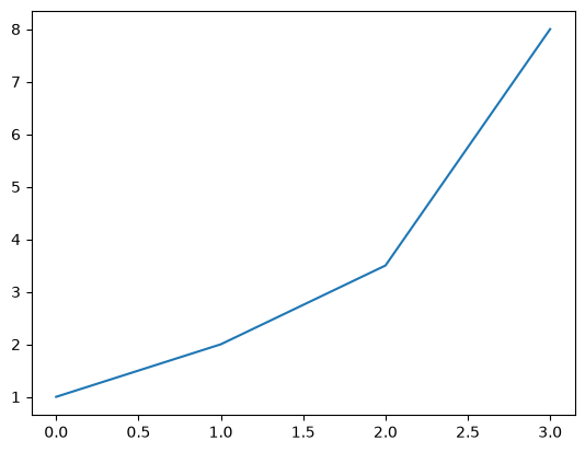
plt.plot([1, 2, 3.5, 8])
[<matplotlib.lines.Line2D at 0x7f93ddd55350>]
Note
Note how matplotlib returns an object representing the plotted data. To avoid displaying the textual representation of this object and keep your notebooks clean, simply assign it to a “throwaway variable”:
_ = plt.plot([1, 2, 3.5, 8])
Scatter plot#
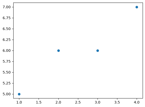
_ = plt.scatter([1, 2, 3, 4], [5, 6, 6, 7])
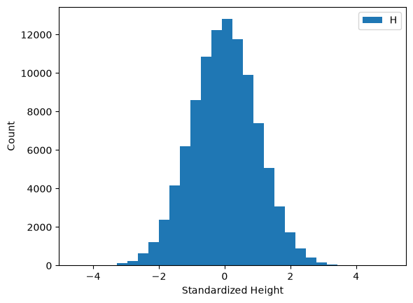
Histogram#
array = np.random.randn(int(10e4)) # random numbers from normal distribution
plt.hist(array, bins=30)  # works with lists as well as numpy arrays
plt.ylabel("Count")
plt.xlabel("Standardized Height")
_ = plt.legend("Height Counts")
Object-oriented Examples#
This time, we will start things off by instantiating the Figure object using matplotlib’s subplots() function:
fig, ax = plt.subplots()
A figure is the “complete” plot, which can contain many subplots, and the axis is the “container” for data itself.
Figures and axes can also be created separately the following two lines:
fig = plt.figure()
ax = fig.add_subplot(111)
Multiple plots#
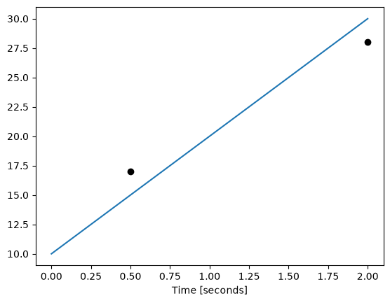
fig, ax = plt.subplots()
ax.plot([10, 20, 30])
ax.scatter([0.5, 2], [17, 28], color='k')
_ = ax.set_xlabel('Time [seconds]')  # the two objects inside the axis object have the same scale
To save a plot we could use the Figure object’s savefig() method:
fig.savefig("scattered.pdf", dpi=300, transparent=True)
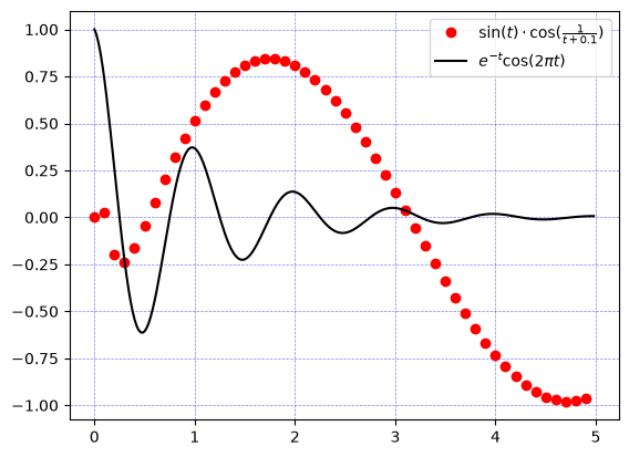
matplotlib is used in conjuction with numpy to visualize arrays:
def f(t):
    return np.exp(-t) * np.cos(2 * np.pi * t)


def g(t):
    return np.sin(t) * np.cos(1 / (t + 0.1))


t1 = np.arange(0.0, 5.0, 0.1)  # (start, stop, step)
t2 = np.arange(0.0, 5.0, 0.02)

# Create figure and axis
fig2 = plt.figure()
ax1 = fig2.add_subplot(111)

# Plot g over t1 and f over t2 in one line
ax1.plot(t1, g(t1), 'ro', t2, f(t2), 'k')

# Add grid
ax1.grid(color='b', alpha=0.5, linestyle='dashed', linewidth=0.5)

# Assigning labels and creating a legend
f_label = r'$e^{-t}\cos(2 \pi t)$'  # Using r'' allows us to use "\" in our strings
g_label = r'$\sin(t) \cdot \cos(\frac{1}{t + 0.1})$'
_ = ax1.legend([g_label, f_label])
Multiple Axes#
data = np.random.randn(2, 1_000)

fig, axs = plt.subplots(2, 2, figsize=(10, 6))  # 4 axes in a 2-by-2 grid.
axs[0, 0].hist(data[0])
axs[1, 0].scatter(data[0], data[1], alpha=0.25)
axs[0, 1].plot(data[0], data[1], '-.', linewidth=0.15)
_ = axs[1, 1].hist2d(data[0], data[1])
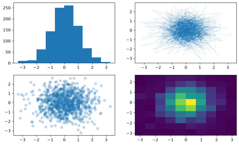
Note that “axes” is a numpy.ndarray instance, and that in order to draw on a specific axis (plot), we start by calling the specific axis according to it’s location on the array.
type(axs)
numpy.ndarray
type(axs[0,0])
matplotlib.axes._subplots.AxesSubplot
# when we want to plot:
axs[<row>,<col>].plot(...)
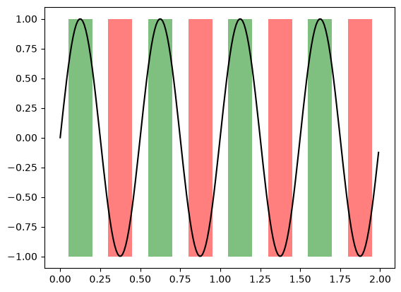
fig, ax = plt.subplots()

x = np.arange(0.0, 2, 0.01)
y = np.sin(4 * np.pi * x)

# Plot line
ax.plot(x, y, color='black')

# Plot patches
ax.fill_between(x, -1, 1, where=y > 0.5, facecolor='green', alpha=0.5)
_ = ax.fill_between(x, -1, 1, where=y < -0.5, facecolor='red', alpha=0.5)
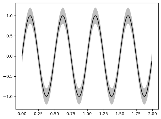
fig, ax = plt.subplots()

x = np.arange(0.0, 2, 0.01)
y = np.sin(4 * np.pi * x)

std = 0.2
y_top = y + std
y_bot = y - std

# Plot line
ax.plot(x, y, color='black')

# Plot STD margin
_ = ax.fill_between(x, y_bot, y_top, facecolor='gray', alpha=0.5)
Using matplotlib’s style objects open up a world of possibilities.
To display available predefined styles:
print(plt.style.available)
['Solarize_Light2', 'bmh', 'classic', 'dark_background', 'fast', 'fivethirtyeight', 'ggplot', 'grayscale', 'petroff10', 'petroff6', 'petroff8', 'seaborn-v0_8', 'seaborn-v0_8-bright', 'seaborn-v0_8-colorblind', 'seaborn-v0_8-dark', 'seaborn-v0_8-dark-palette', 'seaborn-v0_8-darkgrid', 'seaborn-v0_8-deep', 'seaborn-v0_8-muted', 'seaborn-v0_8-notebook', 'seaborn-v0_8-paper', 'seaborn-v0_8-pastel', 'seaborn-v0_8-poster', 'seaborn-v0_8-talk', 'seaborn-v0_8-ticks', 'seaborn-v0_8-white', 'seaborn-v0_8-whitegrid', 'tableau-colorblind10']
Usage example:
plt.style.use('bmh')
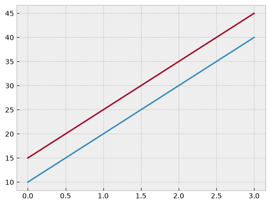
fig, ax = plt.subplots()
ax.plot([10, 20, 30, 40])
_ = ax.plot([15, 25, 35, 45])
SciPy#
SciPy is a large library consisting of many smaller modules, each targeting a single field of scientific computing.
Available modules include scipy.stats, scipy.linalg, scipy.fftpack, scipy.signal and many more.
Because of its extremely wide scope of available use-cases, we won’t go through all of them. All you need to do is to remember that many functions that you’re used to find in different MATLAB toolboxes are located somewhere in SciPy.
Below you’ll find a few particularly interesting use-cases.
.mat files input\output#
from scipy import io as spio

a = np.ones((3, 3))

spio.savemat('file.mat', {'a': a})  # savemat expects a dictionary

data = spio.loadmat('file.mat')
data
{'__header__': b'MATLAB 5.0 MAT-file Platform: posix, Created on: Mon Jun 29 10:43:59 2026',
 '__version__': '1.0',
 '__globals__': [],
 'a': array([[1., 1., 1.],
        [1., 1., 1.],
        [1., 1., 1.]])}
Linear algebra#
from scipy import linalg

# Singular Value Decomposition
arr = np.arange(9).reshape((3, 3)) + np.diag([1, 0, 1])
uarr, spec, vharr = linalg.svd(arr)

# Inverse of square matrix
arr = np.array([[1, 2], [3, 4]])
iarr = linalg.inv(arr)
Curve fitting#
from scipy import optimize


def test_func(x, a, b):
    return a * np.sin(b * x)


# Create noisy data
x_data = np.linspace(-5, 5, num=50)
y_data = 2.9 * np.sin(1.5 * x_data) # create baseline - sin wave
y_data += np.random.normal(size=50) # add normally-distributed noise

fig, ax = plt.subplots()
ax.scatter(x_data, y_data)

params, params_covariance = optimize.curve_fit(test_func,
                                               x_data,
                                               y_data,
                                               p0=[3, 1])
_ = ax.plot(x_data, test_func(x_data, params[0], params[1]), 'k')
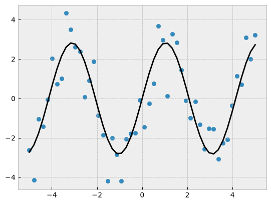
print(params)
[2.82588242 1.51702263]
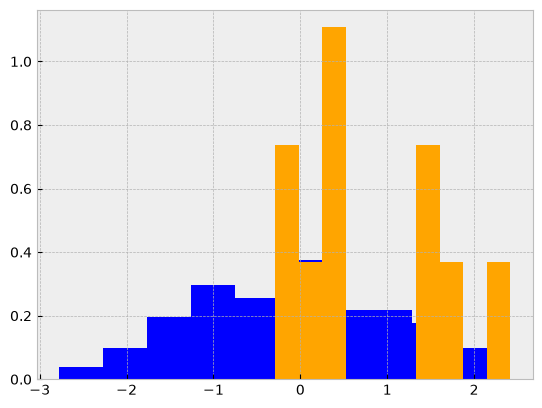
Statistics#
from scipy import stats

# Create two random normal distributions with different paramters
a = np.random.normal(loc=0, scale=1, size=100)
b = np.random.normal(loc=1, scale=1, size=10)

# Draw histograms describing the distributions
fig, ax = plt.subplots()
ax.hist(a, color='blue', density=True)
ax.hist(b, color='orange', density=True)

# Calculate the T-test for the means of two independent samples of scores
stats.ttest_ind(a, b)
TtestResult(statistic=np.float64(-2.4351355021460175), pvalue=np.float64(0.016523706323548305), df=np.float64(108.0))
IPython#
IPython is the REPL in which this text is written in. As stated, it’s the most popular “command window” of Python. When most Python programmers wish to write and execute a small Python script, they won’t use the regular Python interpreter, accessible with python my_file.py. Instead, they will run it with IPython since it has more features. For instance, the popular MATLAB feature which saves the variables that returned from the script you ran is accessible when running a script as ipython -i my_file.py.
Let’s examine some of IPython’s other features, accessible by using the % magic operator before writing your actual code:
%%timeit - micro-benchmarking#
Time execution of a Python statement or expression.
def loop_and_sum(lst):
    """ Loop and some a list """
    sum = 0
    for item in lst:
        sum += item
%timeit loop_and_sum([1, 2, 3, 4, 5])
194 ns ± 1.28 ns per loop (mean ± std. dev. of 7 runs, 10,000,000 loops each)
%timeit loop_and_sum(list(range(10000)))
360 μs ± 2.45 μs per loop (mean ± std. dev. of 7 runs, 1,000 loops each)
%%prun - benchmark each function line#
Run a statement through the python code profiler.
%%prun
data1 = np.arange(500000)
data2 = np.zeros(500000)
ans = data1 + data2 + data1 * data2
loop_and_sum(list(np.arange(10000)))
data1 @ data2
          7 function calls in 0.018 seconds

   Ordered by: internal time

   ncalls  tottime  percall  cumtime  percall filename:lineno(function)
        1    0.015    0.015    0.018    0.018 <string>:1(<module>)
        2    0.002    0.001    0.002    0.001 {built-in method numpy.arange}
        1    0.001    0.001    0.001    0.001 <ipython-input-19-aecde78c78c4>:1(loop_and_sum)
        1    0.000    0.000    0.018    0.018 {built-in method builtins.exec}
        1    0.000    0.000    0.000    0.000 {built-in method numpy.zeros}
        1    0.000    0.000    0.000    0.000 {method 'disable' of '_lsprof.Profiler' objects}
%run - run external script#
Run the named file inside IPython as a program.
%run import_demonstration/my_app/print_the_time.py
1782729858.9250112
%matplotlib [notebook\inline]#
Easily display matplotlib figures inside the notebook and set up matplotlib to work interactively.
%reset#
Resets the namespace by removing all names defined by the user, if called without arguments, or by removing some types of objects, such as everything currently in IPython’s In[] and Out[] containers (see the parameters for details).
LaTeX support#
Render the cell as \(\LaTeX\):
\(a^2 + b^2 = c^2\)
\(e^{i\pi} + 1 = 0\)
scikit-image#
scikit-image is one of the main image processing libraries in Python. We’ll look at it in greater interest later in the semester, but for now let’s examine some of its algorithms:
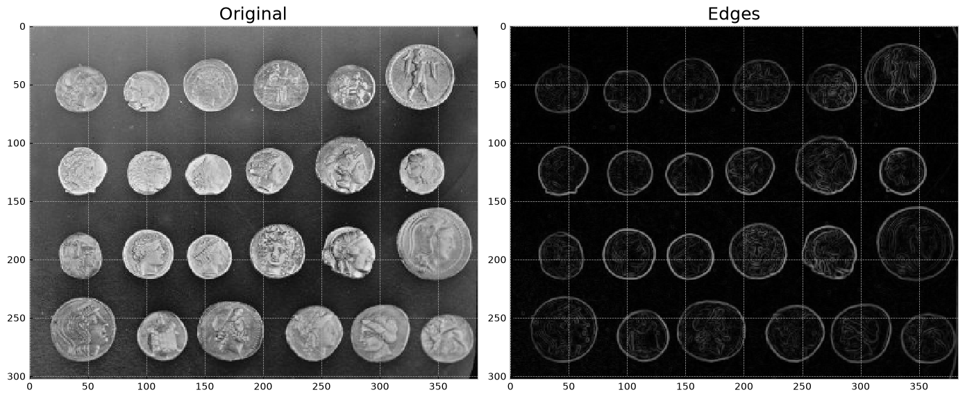
Edge detection using a Sobel filter.#
from skimage import data, io, filters

fig,axes = plt.subplots(1 ,2 ,figsize=(14, 6))

# Plot original image
image = data.coins()
io.imshow(image,ax=axes[0])
axes[0].set_title("Original", fontsize=18)

# Plot edges
edges = filters.sobel(image)  # edge-detection filter
io.imshow(edges,ax=axes[1])
axes[1].set_title("Edges",fontsize=18)

plt.tight_layout()
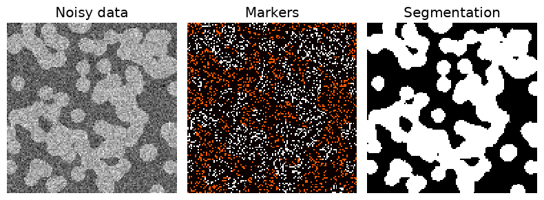
Segmentation using a “random walker” algorithm#
Further reading
The random walker algorithm determines the segmentation of an image from a set of markers labeling several phases (2 or more). An anisotropic diffusion equation is solved with tracers initiated at the markers’ position. The local diffusivity coefficient is greater if neighboring pixels have similar values, so that diffusion is difficult across high gradients. The label of each unknown pixel is attributed to the label of the known marker that has the highest probability to be reached first during this diffusion process.
In this example, two phases are clearly visible, but the data are too noisy to perform the segmentation from the histogram only. We determine markers of the two phases from the extreme tails of the histogram of gray values, and use the random walker for the segmentation.
from skimage.segmentation import random_walker
from skimage.data import binary_blobs
import skimage

# Generate noisy synthetic data
data1 = skimage.img_as_float(binary_blobs(length=128))  # data
data1 += 0.35 * np.random.randn(*data1.shape)  # added noise
markers = np.zeros(data1.shape, dtype=np.uint)
markers[data1 < -0.3] = 1
markers[data1 > 1.3] = 2

# Run random walker algorithm
labels = random_walker(data1, markers, beta=10, mode='bf')

# Plot results
fig, (ax1, ax2, ax3) = plt.subplots(1,
                                    3,
                                    figsize=(8, 3.2),
                                    sharex=True,
                                    sharey=True)
ax1.imshow(data1, cmap='gray', interpolation='nearest')
ax1.axis('off')
ax1.set_adjustable('box')
ax1.set_title('Noisy data')
ax2.imshow(markers, cmap='hot', interpolation='nearest')
ax2.axis('off')
ax2.set_adjustable('box')
ax2.set_title('Markers')
ax3.imshow(labels, cmap='gray', interpolation='nearest')
ax3.axis('off')
ax3.set_adjustable('box')
ax3.set_title('Segmentation')

fig.tight_layout()
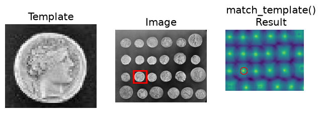
Template matching#
Further reading
We use template matching to identify the occurrence of an image patch (in this case, a sub-image centered on a single coin). Here, we return a single match (the exact same coin), so the maximum value in the match_template result corresponds to the coin location. The other coins look similar, and thus have local maxima; if you expect multiple matches, you should use a proper peak-finding function.
The match_template() function uses fast, normalized cross-correlation 1 to find instances of the template in the image. Note that the peaks in the output of match_template() correspond to the origin (i.e. top-left corner) of the template.
from skimage.feature import match_template

# Extract original coin image
image = skimage.data.coins()
coin = image[170:220, 75:130]

# Find match
result = match_template(image, coin)
ij = np.unravel_index(np.argmax(result), result.shape)
x, y = ij[::-1]

# Create figure and subplots
fig = plt.figure(figsize=(8, 3))
ax1 = plt.subplot(1, 3, 1)
ax2 = plt.subplot(1, 3, 2, adjustable='box')
ax3 = plt.subplot(1, 3, 3, sharex=ax2, sharey=ax2, adjustable='box')

# Plot original coin
ax1.imshow(coin, cmap=plt.cm.gray)
ax1.set_axis_off()
ax1.set_title('Template')

# Plot original image
ax2.imshow(image, cmap=plt.cm.gray)
ax2.set_axis_off()
ax2.set_title('Image')
# (highlight matched region)
hcoin, wcoin = coin.shape
rect = plt.Rectangle((x, y),
                     wcoin,
                     hcoin,
                     edgecolor='r',
                     facecolor='none',
                     linewidth=2)
ax2.add_patch(rect)

# Plot the result of match_template()
ax3.imshow(result)
ax3.set_axis_off()
ax3.set_title('match_template()\nResult')
# (highlight matched region)
ax3.autoscale(False)
_ = ax3.plot(x, y, 'o', markeredgecolor='r', markerfacecolor='none', markersize=10)
Exercise: matplotlib’s Object-oriented Interface#
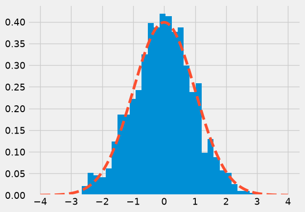
Create 1000 normally-distributed points. Histogram them. Overlay the histogram with a dashed line showing the theoretical normal distribution we would expect from the data.
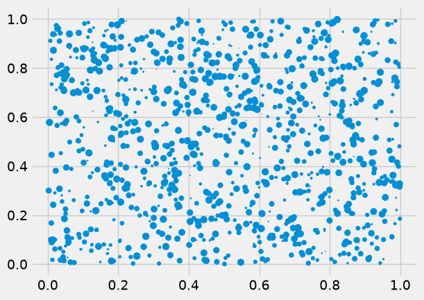
Create a (1000, 3)-shaped matrix of uniformly distributed points between [0, 1). Create a scatter plot with the first two columns as the \(x\) and \(y\) columns, while the third should control the size of the created point.
Using
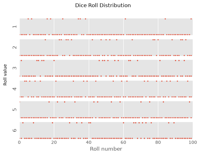
np.random.choice, “roll a die” 100 times. Create a 6x1 figure panel with a shared \(x\)-axis containing values between 0 and 10000 (exclusive). The first panel should show a vector with a value of 1 everywhere the die roll came out as 1, and 0 elsewhere. The second panel should show a vector with a value of 1 everywhere the die roll came out as 2, and 0 elsewhere, and so on. Create a title for the entire figure. The \(y\)-axis of each panel should indicate the value this plot refers to.
Data Analysis with pandas#

A large part of what makes Python so popular nowadays is pandas, or the “Python data analysis library”.
pandas has been around since 2008, and while in itself it’s built on the solid foundations of numpy, it introduced a vast array of important features that can hardly be found anywhere outside of the Python ecosystem. If you can’t find a function that does what you’re trying to do in the documentation, there’s probably a StackOverflow answer or blog-post somewhere with a proposed implementation. Frankly, if you can’t find even that, it might be a good time to stop and make sure you 100% understand what you’re trying to do and why the implementation you have in mind is the “correct” way to do it. Only when and if you reach a positive conclusion, implement it yourself.
The general priniciple in working with pandas is to first look up in its immense codebase (via its docs). or somewhere online, an existing function that does exactly what you’re looking for, and if you can’t - only then should you implement it youself.
Much of the discussion below is taken from the Python Data Science Handbook, by Jake VanderPlas. Be sure to check it out if you need further help with one of the topics.
The need for pandas#
With only clean data in the world, pandas wouldn’t be as necessary. By clean we mean that all of our data was sampled properly, without any missing data points. We also mean that the data is homogeneous, i.e. of a single type (floats, ints), and one-dimensional.
An example of this simple data might be an electrophysiological measurement of a neuron’s votlage over time, a calcium trace of a single imaged neuron and other simple cases such as these.
pandas provide flexibility for our numerical computing tasks via its two main data types: DataFrame and Series, which are multi-puporse data containers with very useful features, which you’ll soon learn about.
Mastering pandas is one of the most important goals of this course. Your work as scientists will be greatly simplified if you’ll feel comfortable in the pandas jungle.
Series#
A pandas Series is generalization of a simple numpy array. It’s the basic building block of pandas objects.
import numpy as np
import pandas as pd  # customary import
import matplotlib.pyplot as plt
series = pd.Series([50., 100., 150., 200.], name='ca_cell1')
# the first argument is the data argument, list-like, just like for numpy

print(f"The output:\n{series}\n")
print(f"Its class:\n{type(series)}")
The output:
0     50.0
1    100.0
2    150.0
3    200.0
Name: ca_cell1, dtype: float64

Its class:
<class 'pandas.Series'>
We received a series instance with our values and an associated index. The index was given automatically, and it defaults to ordinal numbers. Notice how the data is displayed as a column. This is because the pandas library deals with tabular data.
We can access the internal arrays, data and indices, by using the array and index attributes:
series.array # a PandasArray is almost always identical to a numpy array (it's a wrapper)
<NumpyExtensionArray>
[50.0, 100.0, 150.0, 200.0]
Length: 4, dtype: float64
Note that in many places you’ll see series.values used when trying to access the raw data. This is no longer encouraged, and you should generally use either series.array or, even better, series.to_numpy().
series.index # special pandas index object
RangeIndex(start=0, stop=4, step=1)
The index of the array is a true index, just like that of a dictionary, making item access pretty intuitive:
series[1]
np.float64(100.0)
series[:3] # non-inclusive index
0     50.0
1    100.0
2    150.0
Name: ca_cell1, dtype: float64
While this feature is very similar to a numpy array’s index, a series can also have non-integer indices:
data = pd.Series([1, 2, 3, 4], index=['a', 'b', 'c', 'd'])
data
a    1
b    2
c    3
d    4
dtype: int64
data['c'] # as expected
np.int64(3)
data2 = pd.Series(10, index=['first', 'second', 'third'])
data2
first     10
second    10
third     10
dtype: int64
The index of a series is one of its most important features. It also strengthens the analogy of a series to an enhanced Python dictionary. The main difference between a series and a dictionary lies in its vectorization - data inside a series can be processed in a vectorized manner, just like you would act upon a standard numpy array.
Series Instantiation#
Simplest form:
series = pd.Series([1, 2, 3])
series  # indices and dtype inferred
0    1
1    2
2    3
dtype: int64
Or, very similarly:
series = pd.Series(np.arange(10, 20, dtype=np.uint8))
series
0    10
1    11
2    12
3    13
4    14
5    15
6    16
7    17
8    18
9    19
dtype: uint8
Indices can be specified, as we’ve seen:
series = pd.Series(['a', 'b', 'c'], index=['A', 'B', 'C'])
series  # dtype is "object", due to the underlying numpy array
A    a
B    b
C    c
dtype: str
A series (and a DataFrame) can be composed out of a dictionary as well:
continents = dict(Europe=10, Africa=21, America=9, Asia=9, Australia=19)
continents_series = pd.Series(continents)
print(f"Dictionary:\n{continents}\n")
print(f"Series:\n{continents_series}")
Dictionary:
{'Europe': 10, 'Africa': 21, 'America': 9, 'Asia': 9, 'Australia': 19}

Series:
Europe       10
Africa       21
America       9
Asia          9
Australia    19
dtype: int64
Notice how the right dtype was inferred automatically.
When creating a series from a dictionary, the importance of the index is revealed again:
series_1 = pd.Series({'a': 1, 'b': 2, 'c': 3}, index=['a', 'b'])
print(f"Indices override the data:\n{series_1}\n")

series_2 = pd.Series({'a': 1, 'b': 2, 'c': 3}, index=['a', 'b', 'c', 'd'])
print(f"Missing indices will be interpreted as NaNs:\n{series_2}")
Indices override the data:
a    1
b    2
dtype: int64

Missing indices will be interpreted as NaNs:
a    1.0
b    2.0
c    3.0
d    NaN
dtype: float64
We can also use slicing on these non-numeric indices:
print(continents_series)
print("-----")
continents_series['America':'Australia']
Europe       10
Africa       21
America       9
Asia          9
Australia    19
dtype: int64
-----
America       9
Asia          9
Australia    19
dtype: int64
Note
Note the inclusive last index - string indices are inclusive on both ends. This makes more sense when using location-based indices, since in day-to-day speak we regulary talk with “inclusive” indices - “hand me over the tests of students 1-5” obviously refers to 5 students, not 4.
We’ll dicuss pandas indexing extensively later on, but I do want to point out now that indexes can be non-unique:
series = pd.Series(np.arange(5), index=[1, 1, 2, 2, 3])
series
1    0
1    1
2    2
2    3
3    4
dtype: int64
A few operations require a unique index, making them raise an exception, but most operations should work seamlessly.
Lastly, series objects can have a name attached to them as well:
named_series = pd.Series([1, 2, 3], name='Data')
unnamed_series = pd.Series([2, 3, 4])
unnamed_series.rename("Unnamed")
0    2
1    3
2    4
Name: Unnamed, dtype: int64
DataFrame#
A DataFrame is a concatenation of multiple Series objects that share the same index. It’s a generalization of a two dimensional numpy array.
You can also think of it as a dictionary of Series objects, as a database table, or a spreadsheet.
Due to its flexibility, DataFrame is the more widely used data structure.
# First we define a second series
populations = pd.Series(
    dict(Europe=100., Africa=907.8, America=700.1, Asia=2230., Australia=73.7)
)
populations
Europe        100.0
Africa        907.8
America       700.1
Asia         2230.0
Australia      73.7
dtype: float64
olympics = pd.DataFrame({'population': populations, 'medals': continents})
print(olympics)
print(type(olympics))
           population  medals
Europe          100.0      10
Africa          907.8      21
America         700.1       9
Asia           2230.0       9
Australia        73.7      19
<class 'pandas.DataFrame'>
A dataframe has a row index (“index”) and a column index (“columns”):
print(f"Index:\t\t{olympics.index}")
print(f"Columns:\t{olympics.columns}")  # new
Index:		Index(['Europe', 'Africa', 'America', 'Asia', 'Australia'], dtype='str')
Columns:	Index(['population', 'medals'], dtype='str')
Instantiation#
Creating a dataframe can be done in one of several ways:
Dictionary of 1D numpy arrays, lists, dictionaries or Series
A 2D numpy array
A Series
A different dataframe
Alongside the data itself, you can pass two important arguments to the constructor:
columns- An iterable of the headers of each data column.index- Similar to a series.
Just like in the case of the series, passing these arguments ensures that the resulting dataframe will contain these specific columns and indices, which might lead to NaNs in certain rows and\or columns.
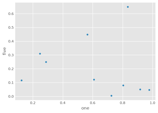
d = {
    'one': pd.Series([1., 2., 3.], index=['a', 'b', 'c']),
    'two': pd.Series([1., 2., 3., 4.], index=['a', 'b', 'c', 'd'])
}

df = pd.DataFrame(d)
df
| one | two | |
|---|---|---|
| a | 1.0 | 1.0 |
| b | 2.0 | 2.0 |
| c | 3.0 | 3.0 |
| d | NaN | 4.0 |
Again, rows will be dropped for missing indices:
pd.DataFrame(d, index=['d', 'b', 'a'])
| one | two | |
|---|---|---|
| d | NaN | 4.0 |
| b | 2.0 | 2.0 |
| a | 1.0 | 1.0 |
A column of NaNs is forced in the case of a missing column:
pd.DataFrame(d, index=['d', 'b', 'a'], columns=['two', 'three'])
| two | three | |
|---|---|---|
| d | 4.0 | NaN |
| b | 2.0 | NaN |
| a | 1.0 | NaN |
A 1D dataframe is also possible:
df1d = pd.DataFrame([1, 2, 3], columns=['data'])
# notice the iterable in the columns argument

df1d
| data | |
|---|---|
| 0 | 1 |
| 1 | 2 |
| 2 | 3 |
df_from_array = pd.DataFrame((np.random.random((2, 10))))
df_from_array
| 0 | 1 | 2 | 3 | 4 | 5 | 6 | 7 | 8 | 9 | |
|---|---|---|---|---|---|---|---|---|---|---|
| 0 | 0.175081 | 0.519184 | 0.464011 | 0.859430 | 0.798958 | 0.683474 | 0.236658 | 0.929695 | 0.949023 | 0.697839 |
| 1 | 0.350483 | 0.781593 | 0.157166 | 0.401172 | 0.289073 | 0.689088 | 0.885764 | 0.823464 | 0.793023 | 0.382852 |
Columnar Operations#
If we continue with the dictionary analogy, we can observe how intuitive the operations on series and dataframe columns can be:
olympics
| population | medals | |
|---|---|---|
| Europe | 100.0 | 10 |
| Africa | 907.8 | 21 |
| America | 700.1 | 9 |
| Asia | 2230.0 | 9 |
| Australia | 73.7 | 19 |
A dataframe can be thought of as a dictionary. Thus, accessing a column is done in the following manner:
olympics['population'] # a column of a dataframe is a series object
Europe        100.0
Africa        907.8
America       700.1
Asia         2230.0
Australia      73.7
Name: population, dtype: float64
This will definitely be one of your main sources of confusion - in a 2D array, arr[0] will return the first row. In a dataframe, df['col0'] will return the first column. Thus, the dictionary analogy might be better suited for indexing operations.
To show a few operations on a dataframe, let’s remind ourselves of the df variable:
df
| one | two | |
|---|---|---|
| a | 1.0 | 1.0 |
| b | 2.0 | 2.0 |
| c | 3.0 | 3.0 |
| d | NaN | 4.0 |
First we see that we can access columns using standard dot notation as well (although it’s usually not recommended):
df.one
a    1.0
b    2.0
c    3.0
d    NaN
Name: one, dtype: float64
Can you guess what will these two operations do?
df['three'] = df['one'] * df['two']
df['flag'] = df['one'] > 2
print(df)
Columns can be deleted with del, or popped like a dictionary:
three = df.pop('three')
three
a    1.0
b    4.0
c    9.0
d    NaN
Name: three, dtype: float64
Insertion of some scalar value will propagate throughout the column:
df['foo'] = 'bar'
df
| one | two | flag | foo | |
|---|---|---|---|---|
| a | 1.0 | 1.0 | False | bar |
| b | 2.0 | 2.0 | False | bar |
| c | 3.0 | 3.0 | True | bar |
| d | NaN | 4.0 | False | bar |
Simple plotting#
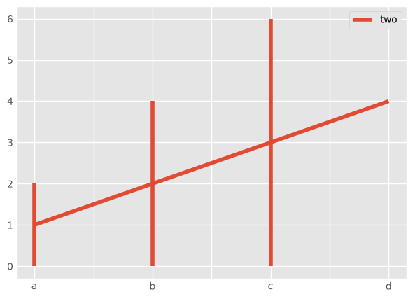
You can plot dataframes and series objects quite easily using the plot() method:
_ = df.plot(kind='line', y='two', yerr='one')
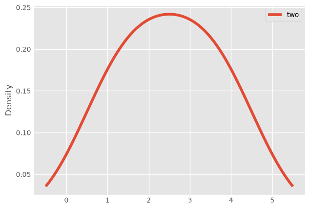
_ = df.plot(kind='density', y='two')
More plotting methods will be shown in class 8.
The assign method#
There’s a more powerful way to insert a column into a dataframe, using the assign method:
olympics_new = olympics.assign(rel_medals=olympics['medals'] /
                               olympics['population'])
olympics_new  # copy of olympics
| population | medals | rel_medals | |
|---|---|---|---|
| Europe | 100.0 | 10 | 0.100000 |
| Africa | 907.8 | 21 | 0.023133 |
| America | 700.1 | 9 | 0.012855 |
| Asia | 2230.0 | 9 | 0.004036 |
| Australia | 73.7 | 19 | 0.257802 |
But assign() can also help us do more complicated stuff:
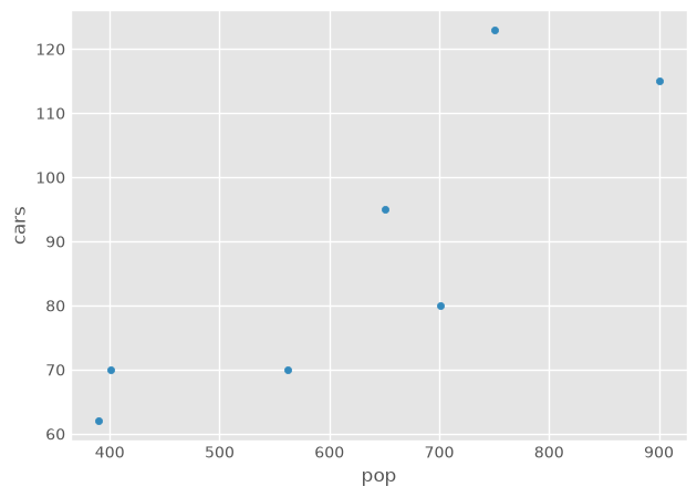
# We create a intermediate dataframe and run the calculations on it
area = [100, 89, 200, 21, 45]
olympics_new["area"] = area
olympics_new.assign(rel_area_medals=lambda x: x.medals / x.area).plot(kind='scatter', x='population', y='rel_area_medals')
plt.show()
print("\nNote that the DataFrame itself didn't change:\n\n",olympics_new)
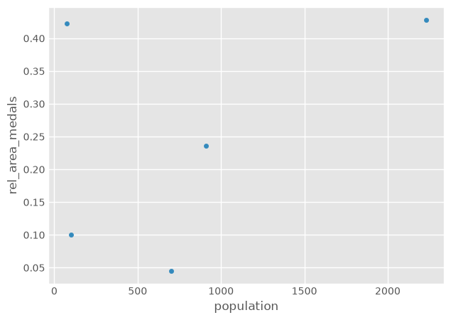
Note that the DataFrame itself didn't change:

            population  medals  rel_medals  area
Europe          100.0      10    0.100000   100
Africa          907.8      21    0.023133    89
America         700.1       9    0.012855   200
Asia           2230.0       9    0.004036    21
Australia        73.7      19    0.257802    45
Note
The lambda expression is an anonymous function (like MATLAB’s @ symbol) and its argument x is the intermediate dataframe we’re handling. A simpler example might look like:
y = lambda x: x + 1
y(3) == 4
Indexing#
pandas indexing can be seem complicated at times due to its high flexibility. However, its relative importance should motivate you to overcome this initial barrier.
The pandas documentation summarizes it in the following manner:
Operation |
Syntax |
Result |
|---|---|---|
Select column |
|
Series |
Select row by label |
|
Series |
Select row by integer location |
|
Series |
Slice rows |
|
DataFrame |
Select rows by boolean vector |
|
DataFrame |
Another helpful summary is the following:
Like lists, you can index by integer position (
df.iloc[intloc]).Like dictionaries, you can index by label (
df[col]ordf.loc[row_label]).Like NumPy arrays, you can index with boolean masks (
df[bool_vec]).Any of these indexers could be scalar indexes, or they could be arrays, or they could be slices.
Any of these should work on the index (=row labels) or columns of a DataFrame.
And any of these should work on hierarchical indexes (we’ll discuss hierarchical indices later).
Let’s see what all the fuss is about:
df
| one | two | flag | foo | |
|---|---|---|---|---|
| a | 1.0 | 1.0 | False | bar |
| b | 2.0 | 2.0 | False | bar |
| c | 3.0 | 3.0 | True | bar |
| d | NaN | 4.0 | False | bar |
.loc#
.loc is primarily label based, but may also be used with a boolean array. .loc will raise KeyError when the items are not found. Allowed inputs are:
A single label, e.g. 5 or ‘a’, (note that 5 is interpreted as a label of the index. This use is not an integer position along the index)
A list or array of labels [‘a’, ‘b’, ‘c’]
A slice object with labels
'a':'f'(note that contrary to usual python slices, both the start and the stop are included, when present in the index! - also see Slicing with labels)A boolean array
A callable function with one argument (the calling Series, DataFrame or Panel) and that returns valid output for indexing (one of the above)
df.loc['a'] # a series is returned
one       1.0
two       1.0
flag    False
foo       bar
Name: a, dtype: object
df.loc['a':'b'] # two items!
| one | two | flag | foo | |
|---|---|---|---|---|
| a | 1.0 | 1.0 | False | bar |
| b | 2.0 | 2.0 | False | bar |
Using characters is always inclusive on both ends. This is because it’s more “natural” this way, according to pandas devs. As natural as it may be, it’s definitely confusing.
df.loc[[True, False, True, False]]
| one | two | flag | foo | |
|---|---|---|---|---|
| a | 1.0 | 1.0 | False | bar |
| c | 3.0 | 3.0 | True | bar |
2D indexing also works:
df.loc['c', 'flag']
np.True_
.iloc#
.iloc is primarily integer position based (from 0 to length-1 of the axis), but may also be used with a boolean array. .iloc will raise IndexError if a requested indexer is out-of-bounds, except slice indexers which allow out-of-bounds indexing. (this conforms with Python/numpy slice semantics). Allowed inputs are:
An integer, e.g.
5A list or array of integers
[4, 3, 0]A slice object with ints
1:7A boolean array
A callable function with one argument (the calling Series, DataFrame or Panel) and that returns valid output for indexing (one of the above)
df.iloc[1:3]
| one | two | flag | foo | |
|---|---|---|---|---|
| b | 2.0 | 2.0 | False | bar |
| c | 3.0 | 3.0 | True | bar |
df.iloc[[True, False, True, False]]
| one | two | flag | foo | |
|---|---|---|---|---|
| a | 1.0 | 1.0 | False | bar |
| c | 3.0 | 3.0 | True | bar |
df
| one | two | flag | foo | |
|---|---|---|---|---|
| a | 1.0 | 1.0 | False | bar |
| b | 2.0 | 2.0 | False | bar |
| c | 3.0 | 3.0 | True | bar |
| d | NaN | 4.0 | False | bar |
2D indexing works as expected:
df.iloc[2, 0]
np.float64(3.0)
We can also slice rows in a more intuitive fashion:
df[1:10]
| one | two | flag | foo | |
|---|---|---|---|---|
| b | 2.0 | 2.0 | False | bar |
| c | 3.0 | 3.0 | True | bar |
| d | NaN | 4.0 | False | bar |
Notice how no exception was raised even though we tried to slice outside the dataframe boundary. This conforms to standard Python and numpy behavior.
This slice notation (without .iloc or .loc) works fine, but it sometimes counter-intuitive. Try this example:
df2 = pd.DataFrame([[1, 2, 3, 4], [5, 6, 7, 8]],
                   columns=['A', 'B', 'C', 'D'],
                   index=[10, 20])
df2
| A | B | C | D | |
|---|---|---|---|---|
| 10 | 1 | 2 | 3 | 4 |
| 20 | 5 | 6 | 7 | 8 |
df2[1:] # we succeed with slicing
| A | B | C | D | |
|---|---|---|---|---|
| 20 | 5 | 6 | 7 | 8 |
df2[1]  # we fail, since the key "1" isn't in the columns
# df2[10] - this also fails
---------------------------------------------------------------------------
KeyError                                  Traceback (most recent call last)
File /opt/hostedtoolcache/Python/3.11.15/x64/lib/python3.11/site-packages/pandas/core/indexes/base.py:3641, in Index.get_loc(self, key)
   3640 try:
-> 3641     return self._engine.get_loc(casted_key)
   3642 except KeyError as err:

File pandas/_libs/index.pyx:168, in pandas._libs.index.IndexEngine.get_loc()
--> 168 'Could not get source, probably due dynamically evaluated source code.'

File pandas/_libs/index.pyx:176, in pandas._libs.index.IndexEngine.get_loc()
--> 176 'Could not get source, probably due dynamically evaluated source code.'

File pandas/_libs/index.pyx:583, in pandas._libs.index.StringObjectEngine._check_type()
--> 583 'Could not get source, probably due dynamically evaluated source code.'

KeyError: 1

The above exception was the direct cause of the following exception:

KeyError                                  Traceback (most recent call last)
Cell In[78], line 1
----> 1 df2[1]  # we fail, since the key "1" isn't in the columns
      2 # df2[10] - this also fails

File /opt/hostedtoolcache/Python/3.11.15/x64/lib/python3.11/site-packages/pandas/core/frame.py:4378, in DataFrame.__getitem__(self, key)
   4374
   4375         if is_single_key:
   4376             if self.columns.nlevels > 1:
   4377                 return self._getitem_multilevel(key)
-> 4378             indexer = self.columns.get_loc(key)
   4379             if is_integer(indexer):
   4380                 indexer = [indexer]
   4381         else:

File /opt/hostedtoolcache/Python/3.11.15/x64/lib/python3.11/site-packages/pandas/core/indexes/base.py:3648, in Index.get_loc(self, key)
   3643     if isinstance(casted_key, slice) or (
   3644         isinstance(casted_key, abc.Iterable)
   3645         and any(isinstance(x, slice) for x in casted_key)
   3646     ):
   3647         raise InvalidIndexError(key) from err
-> 3648     raise KeyError(key) from err
   3649 except TypeError:
   3650     # If we have a listlike key, _check_indexing_error will raise
   3651     #  InvalidIndexError. Otherwise we fall through and re-raise
   3652     #  the TypeError.
   3653     self._check_indexing_error(key)

KeyError: 1
This is why we generally prefer indexing with either .loc or .iloc. We know what we’re after, and we explicitly write it.
Indexing with query and where#
Exercise: Pandas Indexing#
import numpy as np
import pandas as pd
Basics #1
Create a mock
pd.Seriescontaining the number of autonomous cars in different cities in Israel. Use proper naming and datatypes, and have at least 7 data points.
Show the mean, standard deviation and median of the Series.
Create another mock Series with population counts of the cities you used.
Make a DataFrame from both series and plot (scatter plot) the number of autonomous cars as a function of the population using the pandas’ API only, without a direct call to
matplotlib.
Basics #2
Create three random
pd.Seriesand generate apd.DataFramefrom them. Name each series, but make sure to use the same, non-numeric, index for the different series.
Display the underlying
numpyarray.
Create a new column from the addition of two of the columns without the
assign()method.
Create a new column from the multiplication of two of the columns using
assign(), and plot the result.
Take the sine of the entire dataframe.
Dates and times in pandas
Create a DataFrame with at least two columns, a datetime index (look at
pd.date_range) and random data.
---------------------------------------------------------------------------
ValueError                                Traceback (most recent call last)
File pandas/_libs/tslibs/offsets.pyx:6338, in pandas._libs.tslibs.offsets.to_offset()
-> 6338 'Could not get source, probably due dynamically evaluated source code.'

File pandas/_libs/tslibs/offsets.pyx:6205, in pandas._libs.tslibs.offsets._validate_to_offset_alias()
-> 6205 'Could not get source, probably due dynamically evaluated source code.'

ValueError: 'M' is no longer supported for offsets. Please use 'ME' instead.

During handling of the above exception, another exception occurred:

ValueError                                Traceback (most recent call last)
Cell In[89], line 1
----> 1 dates = pd.date_range(start='20180101', periods=6, freq='M')
      2 dates  # examine the dates we were given

File /opt/hostedtoolcache/Python/3.11.15/x64/lib/python3.11/site-packages/pandas/core/indexes/datetimes.py:1442, in date_range(start, end, periods, freq, tz, normalize, name, inclusive, unit, **kwargs)
   1440     freq = "D"
   1441 if freq is not None:
-> 1442     freq = to_offset(freq)
   1444 if start is NaT or end is NaT:
   1445     # This check needs to come before the `unit = start.unit` line below
   1446     raise ValueError("Neither `start` nor `end` can be NaT")

File pandas/_libs/tslibs/offsets.pyx:6254, in pandas._libs.tslibs.offsets.to_offset()
-> 6254 'Could not get source, probably due dynamically evaluated source code.'

File pandas/_libs/tslibs/offsets.pyx:6377, in pandas._libs.tslibs.offsets.to_offset()
-> 6377 'Could not get source, probably due dynamically evaluated source code.'

File pandas/_libs/tslibs/offsets.pyx:6162, in pandas._libs.tslibs.offsets.raise_invalid_freq()
-> 6162 'Could not get source, probably due dynamically evaluated source code.'

ValueError: Invalid frequency: M. Failed to parse with error message: ValueError("'M' is no longer supported for offsets. Please use 'ME' instead.")
Convert the dtype of one of the columns (int <-> float).
---------------------------------------------------------------------------
AttributeError                            Traceback (most recent call last)
Cell In[91], line 1
----> 1 df.A = df.A.astype(int)

File /opt/hostedtoolcache/Python/3.11.15/x64/lib/python3.11/site-packages/pandas/core/generic.py:6194, in NDFrame.__getattr__(self, name)
   6190             and name not in self._accessors
   6191             and self._info_axis._can_hold_identifiers_and_holds_name(name)
   6192         ):
   6193             return self[name]
-> 6194         return object.__getattribute__(self, name)

AttributeError: 'DataFrame' object has no attribute 'A'
View the top and bottom of the dataframe using the head and tail methods. Make sure to visit describe() as well.
Use the
sort_valueby column values to sort your dataframe. What happened to the indices?
Re-sort the dataframe with the sort_index method.
Display the value in the third row, at the second column. What is the most well suited indexing method?
DataFrame comparisons and operations
Generate another DataFrame with at least two columns. Populate it with random values between -1 and 1.
Find the places where the dataframe contains negative values, and replace them with their positive inverse (-0.21 turns to 0.21).
Set one of the values to NaN using
.loc.
Drop the entire column containing this null value.