Class 5: The Scientific Stack - Part I: numpy#
Scientific Python#
Introduction#

The onion-like scientific stack of Python is composed of the most important packages used in the Python scientific world. Here’s a quick overview of the most important names in the stack, before we dive in deep:
IPython: A REPL, much like the command window in MATLAB. Lets you write Python on the fly, debug and check the performance of your code, and much (much!) more.
Jupyter: Notebooks designed for data exploration. Write code and see its output immediately, with useful rich text (Markdown) annotations to accompany it (just like this notebook!).
NumPy: Standard implementation of multi-dimensional arrays in Python.
pandas: Tabular data manipulation.
SciPy: Implements advanced algorithms widely used in scientific programming, including advanced linear algebra, data structures, curve fitting, signal processing, modeling and more.
matplotlib: A cornerstone for data visualization in Python.
seaborn: Smart visualizations of tabular data.
This scientific stack is one of the main reasons that empowered Python in recent years to the prominent role it has today. Throughout the course you will become familiar with all of the aforementioned tools, and more.
NumPy#
NumPy is the de-facto implementation of arrays in Python. They’re very similar to MATLAB arrays (and to other implementations in other programming languages).
Although numpy is used extensively in the Python eco-system, it doesn’t come with the Python standard library, which means you have to install it first. Activate your environment and run pip install numpy from the command line (inside VSCode, for example). Only then you can follow the rest of the class.
import numpy as np  # standard alias for numpy

l = [1, 2, 3]
array = np.array(l)  # obviously same as np.array([1, 2, 3])
array
array([1, 2, 3])
The created array variable is a numpy array. Notice how numpy has to take existing data, in this case in the form of a list (l), and convert it into an array. In MATLAB everything is an array all the time so we don’t think of this conversion, but here the conversion happens explicitly when you call np.array() on some collection of data.
Let’s continue to examine the basic properties of this array:
# Check the dimensionality of the array:
print("Shape:\t", array.shape)
print("NDim:\t", array.ndim)
Shape:	 (3,)
NDim:	 1
We’ve instantiated an array by calling the np.array() function on an iterable. This will create a one-dimensional numpy array, or vector. This is the first important difference from MATLAB. In MATLAB, all arrays are by default n-dimensional. If you write:
a = 1
a(:, :, :, :, :, 1) = 2
then you just received a 6-dimensional array. NumPy doesn’t allow that. The dimensions of an array are generally the dimensions it had when it was created. You can always use reshape(), like MATLAB, to define the exact number of dimensions you wish to have. You can also use newaxis() to add an axis, as we’ll see below. But these options still keep the number of elements in the array the same, they just re-order them.
This means that a 2x4 array can be reshaped into a 4x2 array, or a 2x2x2 one, but not 3x3x3.
The second difference is the idea of vectors.
print(f"The number of dimensions is {array.ndim}.")
print(f"The shape is {array.shape}.")
The number of dimensions is 1.
The shape is (3,).
As you see, ndim returns the number of dimensions. The shape is returned as a tuple, the length of which is the number of dimensions, while the values represent the number of elements in each dimensions. shape is very similar to the size() function of MATLAB.
Note that:
a = np.array(1)  # wrong instatiation! Don't use it, instead write np.array([1])
print("Wrong instantiation results:")
print("Shape: ", a.shape)
print("NDim: ", a.ndim)
Wrong instantiation results:
Shape:  ()
NDim:  0
So be mindful to pass an iterable.
Creating arrays with more than one dimension might look odd at a first glance:
arr_2d = np.array([[1, 2, 3], [4, 5, 6]])
arr_2d
array([[1, 2, 3],
       [4, 5, 6]])
print(f"The number of dimensions is {arr_2d.ndim}.")
print(f"The shape is {arr_2d.shape}.")
print(f"The len of the array is {len(arr_2d)} - which corresponds to the shape of the 0th dimension.")
The number of dimensions is 2.
The shape is (2, 3).
The len of the array is 2 - which corresponds to the shape of the 0th dimension.
As we see, each list was considered a single “row” (dimension number 0) in the final array, very much like MATLAB, although the syntax can be confusing at first. Here’s another slightly confusing example:
c = np.array([[[1], [2]], [[3], [4]]])
c
array([[[1],
        [2]],

       [[3],
        [4]]])
c.shape
(2, 2, 1)
Or, alternatively:
c2 = np.array([1, 2, 3, 4]).reshape((2, 2, 1))
c2.shape
(2, 2, 1)
Creating Arrays#
np.arange(10) # similar to MATLAB's 0:9 (and to Python's range())
array([0, 1, 2, 3, 4, 5, 6, 7, 8, 9])
np.arange(start=1, stop=8, step=3) # MATLAB's 1:3:8
array([1, 4, 7])
np.zeros((2, 3)) # notice that the shape is a tuple
array([[0., 0., 0.],
       [0., 0., 0.]])
np.zeros_like(arr_2d)
array([[0, 0, 0],
       [0, 0, 0]])
np.ones((1, 4), dtype='int64') # 2-d array with the dtype argument
array([[1, 1, 1, 1]])
np.full((4, 2), 7)
array([[7, 7],
       [7, 7],
       [7, 7],
       [7, 7]])
np.linspace(0, 10, 3) # start, stop, number of points (endpoint as a keyword argument)
array([ 0., 5., 10.])
np.linspace(0, 10, 3, endpoint=False, dtype=np.float32) # float32 is "single" in MATLAB-speak. float64, which is the default, is "double"
array([0. , 3.3333333, 6.6666665], dtype=float32)
np.eye(3, dtype='uint8')
array([[1, 0, 0],
       [0, 1, 0],
       [0, 0, 1]], dtype=uint8)
np.diag([19, 20])
array([[19,  0],
       [ 0, 20]])
Some more interesting features:
np.array([True, False, False]) # A logical mask
array([ True, False, False])
np.array([1+2j]).dtype # Complex numbers
dtype('complex128')
np.array(['a', 'bc', 'd', 'e'])
# No such thing as a cell array, arrays can contain strings.
array(['a', 'bc', 'd', 'e'], dtype='<U2')
* <U2 are strings containing maximum 2 unicode letters
Arrays can be heterogeneous, although usually this is discouraged.
To make an hetetogeneous array, you have to specify its data type as object, or np.object:
np.array([1, 'b', True, {'b': 1}], dtype=object)
array([1, 'b', True, {'b': 1}], dtype=object)
The last few examples showed us that NumPy arrays are a superset of MATLAB’s matrices, as they also contain the cell array functionality within them.
When multiplying NumPy arrays, multiplication is done cell-by-cell (elementwise), rather than by the rules of linear algebra.
You can still multiply vectors and matrices using one of two options:
The
@operator (preferred):arr1 @ arr2arr1.dot(arr2)
Just remember that the default behavior is different than MATLAB’s.
Note
NumPy does contain a matrix-like array - np.matrix('1 2; 3 4'), which behaves like a linear algebra 2D matrix (see np.matrix), but its use is discouraged.
More on Datatypes#
Many array creation and handling methods have a dtype keyword argument, that allow you to specify the required output’s data type easily.
Python will issue a RuntimeWarning whenever an “unsafe” conversion of data type will occur, for example from np.float64 to np.float32.
NumPy Arrays vs. Lists#
You might have asked yourselves by this point what’s the difference between lists and numpy arrays. In other words, if Python already has an array-like data structure, why does it need another one?
Lists are truly amazing, but their flexibility comes at a cost. You won’t notice it when you’re writing some short script, but when you start working with real datasets you notice that their performance is lacking.
Naive iteration over lists is good enough when the lists contain up to a few thousands of elements, but somewhere after this invisible threshold you will start to notice the runtimes of your app turning very slow.
Why are lists slower?#
Lists are slower due to their implementation. Because a list has to be heterogeneous, a list is actually an object containing references to other objects, which are the elements of the data contained in the list. This nesting can go on even deeper, since elements of lists can be other lists, or other complex data types.
Iterating over such a complicated objects contains a lot of “overhead”, i.e. time the interpreter tries to figure out what is it actually facing - is this current value an integer? A float? A dictionary of tuples?
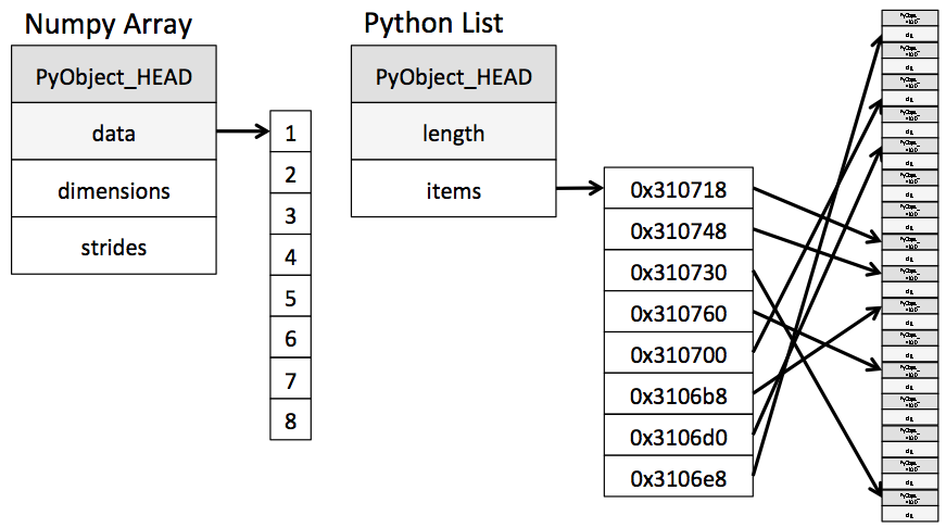
This is where NumPy arrays come into the picture. They require the contained data to be homogeneous (disregarding the “object” datatype), leading to a simpler structure of the underlying implementation: A NumPy array is an object with a pointer to a contiguous block of data in the memory.
NumPy forces the elements in its array to be homogeneous, by means of “upcasting”:
arr = np.array([1, 2, 3.14, 4])
arr  # upcasted to float, not "object", since it's much slower
array([1. , 2. , 3.14, 4. ])
This homogeneity and contiguity allows NumPy to use “vectorized” functions, which are simply functions that can iterate in C code over the array, as opposed to regular functions which have to use the Python iteration rules.
This means that while in essence the following two pieces of code are identical, the performance gain is due to the loop being done in C rather than in Python (this is the case in MATLAB as well):
%%timeit
python_array = list(range(1_000_000))
for item in python_array:
    item += 1
55.4 ms ± 665 µs per loop (mean ± std. dev. of 7 runs, 10 loops each)
%%timeit
numpy_array = np.arange(1_000_000)
numpy_array += 1  # inside, a C loop is adding 1 to each item.

# Two orders of magnitude improvement for a pretty small (1M elements) array.
# This is approximately the size of a 1024x1024 pixel image.
1.67 ms ± 51.2 µs per loop (mean ± std. dev. of 7 runs, 1000 loops each)
If you recall the first class, you’ll remember that we mentioned how Python code has to be transpiled into C code, which is then compiled to machine code. NumPy arrays take a “shortcut” here, are are quickly compiled to efficient C code without the Python overhead. When using vectorized NumPy operations, the loop Python does in the backstage is very similar to a loop that a C programmer would have written by hand.
Another small but significant benefit of NumPy arrays is smaller memory footprint:
from sys import getsizeof

python_array = list(range(1_000_000))
list_size = getsizeof(python_array) / 1e6  # in MB
print(f"Python list size (1M elements, MB): {list_size}")

numpy_array = np.arange(1_000_000, dtype=np.int32)
numpy_size = numpy_array.nbytes / 1e6
print(f"Numpy array size (1M elements, MB): {numpy_size}")
Python list size (1M elements, MB): 8.000056
Numpy array size (1M elements, MB): 4.0
Why do 1 million elements require 4MB?
Each element has to weigh 4 bytes, or 32 bits. This means that the np.arange() function generates by default int32 values.
Lower memory usage can help us pack larger array in the computer’s working memory (RAM), and it will also improve the performance of the underlying code.
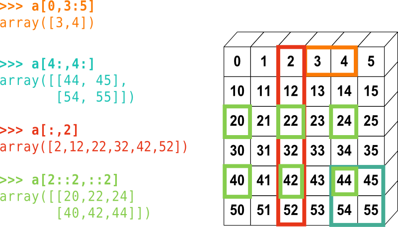
Indexing and Slicing#
Indexing numpy arrays is very much what you’d expect it to be.
a = np.arange(10)
a[0], a[3], a[-2]  # Python indexing is always done with square brackets
(0, 3, 8)
The beautiful reverse slicing works here as well:
a[::-1]
array([9, 8, 7, 6, 5, 4, 3, 2, 1, 0])
arr_2d
array([[1, 2, 3],
       [4, 5, 6]])
arr_2d[0, 2] # first row, third column
3
arr_2d[0, :] # first row, all columns
array([1, 2, 3])
arr_2d[0]  # first item in the first dimension, and all of its corresponding elemets
# Similar to arr_2d[0, :]
array([1, 2, 3])
a[1::2]
array([1, 3, 5, 7, 9])
a[:2] # last index isn't included
array([0, 1])
View vs. Copy#
In Python, slicing creates a view of an object, not a copy:
b = a[::2]
b
array([0, 2, 4, 6, 8])
b[0] = 100
b
array([100, 2, 4, 6, 8])
a # a is also changed!
array([100, 1, 2, 3, 4, 5, 6, 7, 8, 9])
Copying is done with copy():
a_copy = a[::-1].copy()
a_copy
array([ 9, 8, 7, 6, 5, 4, 3, 2, 1, 100])
a_copy[1] = 200
a_copy
array([ 9, 200, 7, 6, 5, 4, 3, 2, 1, 100])
a # unchanged
array([100, 1, 2, 3, 4, 5, 6, 7, 8, 9])
This behavior allows NumPy to save time and memory. It will usually go unnoticed during day-to-day use. Occasionally, however, it can result in ugly bugs which are hard to locate.
Let’s look at a summary of 2D indexing:
Aggregation#
arr = np.random.random(1_000)
sum(arr)  # The native Python sum works on numpy arrays, but its use is discouraged in this context
512.7631727029587
sum() is a built-in Python function, capable of working on lists and other native Python data structures. NumPy has its own sum functions: You can either write np.sum(arr), or use arr.sum():
%timeit sum(arr)
%timeit np.sum(arr)
%timeit arr.sum()
211 µs ± 7.71 µs per loop (mean ± std. dev. of 7 runs, 1000 loops each)
4.39 µs ± 109 ns per loop (mean ± std. dev. of 7 runs, 100000 loops each)
2.87 µs ± 14.3 ns per loop (mean ± std. dev. of 7 runs, 100000 loops each)
Keep in mind that the built-in sum() and numpy’s np.sum() aren’t identical. np.sum() by default calculates the sum of all axes, returning a single number for multi-dimensional arrays.
In MATLAB, this behavior is replicated with sum(arr(:)).
Likewise, min() and max() also have two “competing” versions:
%timeit min(arr)  # Native Python
%timeit np.min(arr)
%timeit arr.min()
125 µs ± 1.54 µs per loop (mean ± std. dev. of 7 runs, 10000 loops each)
4.5 µs ± 61.3 ns per loop (mean ± std. dev. of 7 runs, 100000 loops each)
3.02 µs ± 39.5 ns per loop (mean ± std. dev. of 7 runs, 100000 loops each)
Calculating the min of an array will, again, result in a single number:
arr2 = np.random.random((4, 4, 4))
arr2.min()
0.038580771529663105
If you wish to calculate it across an axis, use the axis keyword:
arr2.min(axis=0)
[[0.07637196 0.11851706 0.05473045 0.07816811]
 [0.09183216 0.06991563 0.28786821 0.36936303]
 [0.09021839 0.03858077 0.12515445 0.10292086]
 [0.41324246 0.18667301 0.1655201  0.46430161]]
2D output (axis number 0 was “dropped”)
arr2.max(axis=(0, 1))
[0.95060274 0.95759997 0.91357163 0.91681919]
1D output (the two first axes were summed over)
Many other aggregation functions exist, including:
- np.var
- np.std
- np.argmin\argmax
- np.median
- ...
Most of them have an object-oriented version, i.e. arr.var(), and a procedural version, i.e. np.var(arr).
Fancy Indexing#
In NumPy, indexing an array with a different array is called “fancy” indexing. Perhaps confusingly, it creates a copy, not a view.
basic_array = np.arange(10)
basic_array
array([0, 1, 2, 3, 4, 5, 6, 7, 8, 9])
mask = basic_array % 2 == 0
mask
---------------------------------------------------------------------------
NameError                                 Traceback (most recent call last)
<ipython-input-1-70b4ebab88b9> in <module>
----> 1 mask = basic_array % 2 == 0
      2 mask

NameError: name 'basic_array' is not defined
b = basic_array[mask]  # same as basic_array[basic_array % 2 == 0]
b
array([0, 2, 4, 6, 8])
MATLAB veterans shouldn’t be surprised from this feature, but if you haven’t seen it before make sure to have a firm grasp on it, as it’s a very powerful technique.
b[:] = 999
print(f"basic array: {basic_array}")
print(f"b: {b}")
basic array: [0 1 2 3 4 5 6 7 8 9]
b: [999 999 999 999 999]
Note basic_array was not changed.
float_array = np.arange(start=0, stop=20, step=1.5)
float_array
array([ 0. ,  1.5,  3. ,  4.5,  6. ,  7.5,  9. , 10.5, 12. , 13.5, 15. ,
       16.5, 18. , 19.5])
float_array[[1, 2, 5, 5, 10]]  # copy, not a view. Meaning that the resulting array is a new
# instance of the original array, independent of it, in a different location in memory.
array([ 1.5, 3. , 7.5, 7.5, 15. ])
Counting the number of values that satisfy some condition can be done using np.count_nonzero() or np.sum():
basic_array = np.arange(10)
count_nonzero_result = np.count_nonzero(basic_array % 2 == 0)
sum_result = np.sum(basic_array % 2 == 0)

print(f"np.count_nonzero result: {count_nonzero_result}")
print(f"np.sum result: {sum_result}")
# In the latter case, True is 1 and False is 0
np.count_nonzero result: 5
np.sum result: 5
If we wish to add more conditions in to the mix, we can use the &, |, ~, ^ operators (and, or, not, xor):
((basic_array % 2 == 1) & (basic_array != 3)).sum() # uneven values that are different from 3
4
Note that numpy uses the &, |, ~, ^ operators for element-by-element comparison, while the reserved and and or keywords evaluate the entire object:
np.sum((basic_array % 2 == 1) and (basic_array != 3)) # doesn't work, "and" isn't used this way here
---------------------------------------------------------------------------
ValueError                                Traceback (most recent call last)
<ipython-input-60-e462a6643cbd> in <module>
----> 1 np.sum((basic_array % 2 == 1) and (basic_array != 3))   # doesn't work, "and" isn't used this way here

ValueError: The truth value of an array with more than one element is ambiguous. Use a.any() or a.all()
Sorting#
Again we face a condition in which Python has its own sort functions, but numpy’s np.sort() are much better suited for arrays. We can either sort in-place, or have a new object back:
# Return a new object:
arr = np.array([ 3, 4, 1, 8, 10, 2, 4])
print(np.sort(arr))

# Sort in-place:
arr.sort()
print(arr)
[ 1  2  3  4  4  8 10]
[ 1  2  3  4  4  8 10]
The default implementation is a quicksort but other sorting algorithms can be found as well.
# np.argsort will return the indices of the sorted array:
arr = np.array([ 3, 4, 1, 8, 10, 2, 4])
print("Sorted indices: {}".format(np.argsort(arr)))

# Usage is as follows:
arr[np.argsort(arr)]
Sorted indices: [2 5 0 1 6 3 4]
array([ 1, 2, 3, 4, 4, 8, 10])
Concatenation#
Concatenation (and splitting) in numpy works as follows:
x = np.array([1, 2, 3])
y = np.array([3, 2, 1])
np.concatenate([x, y])  # concatenates along the first axis
array([1, 2, 3, 3, 2, 1])
# Concatenate more than two arrays
z = [99, 99, 99]
np.concatenate([x, y, z])  # notice how the function argument is an iterable!
array([ 1, 2, 3, 3, 2, 1, 99, 99, 99])
# 2D - along the last axis
twod_1 = np.array([[0, 1, 2],
                   [3, 4, 5]])
twod_2 = np.array([[6, 7, 8],
                   [9, 10, 11]])
np.concatenate((twod_1, twod_2), axis=-1)
array([[ 0,  1,  2,  6,  7,  8],
       [ 3,  4,  5,  9, 10, 11]])
np.vstack() and np.hstack() are also an option:
sim1 = np.array([0, 1, 2])
sim2 = np.array([[30, 40, 50],
                 [60, 70, 80]])
np.vstack((sim1, sim2))
array([[ 0,  1,  2],
       [30, 40, 50],
       [60, 70, 80]])
Splitting up arrays is also quite easy:
arr = np.arange(16).reshape((4, 4))  # see the tuple? Shapes of arrays always come in tuples
arr
array([[ 0,  1,  2,  3],
       [ 4,  5,  6,  7],
       [ 8,  9, 10, 11],
       [12, 13, 14, 15]])
upper, lower = np.split(arr, [3])  # splits at the fourth line (of the first axis, by default)
print(upper)
print('---')
print(lower)
[[ 0  1  2  3]
 [ 4  5  6  7]
 [ 8  9 10 11]]
---
[[12 13 14 15]]
Familiarization Exercise
Create two random 3D arrays, at least 3x3x3 in size. The first should have random integers between 0 and 100, while the second should contain floating points numbers drawn from the normal distribution, with mean -1 and standard deviation of 2
What are the default datatypes of integer and floating-point arrays in NumPy?
Solution
>>> low = 0
>>> high = 100
>>> size = 10, 10, 10
>>> array_1 = np.random.randint(low=low, high=high, size=size)
>>> array_2 = np.random.randn(*size) * 2 - 1
>>> array_1.dtype
dtype('int64')
>>> array_2.dtype
dtype('float64')
Center the distribution of the first integer array around 0, with minimal and maximal values ranging between -1 and 1.
Solution
>>> middle = (array_1.max() - array_1.min()) / 2
>>> centered_array_1 = (array_1 - middle) / middle
Calculate the mean and standard deviation of each array along the last axis, and the sum along the second axis. Use the object-oriented implementation of these functions.
Solution
>>> print("\narray_1 (integers) stats:")
>>> print(f"Mean:\t{array_1.mean()}\nSTD:\n{array_1.std(axis=-1)}\nSum:\n{array_1.sum(axis=1)}")
>>> print("\narray_2 (normal distribution) stats:")
>>> print(f"Mean:\t{array_2.mean()}\nSTD:\n{array_2.std(axis=-1)}\nSum:\n{array_2.sum(axis=1)}")
array_1 (integers) stats:
Mean:   49.025,
STD:
[[27.78920654 29.11717706 20.05218193 32.00312485 26.01326585 29.29573348
  25.86909353 28.75499957 34.52375993 24.20826305]
 [30.57384503 21.83689538 27.17149241 25.25787006 35.64112793 21.12912682
  14.4374513  23.75731466 29.45318319 31.1409698 ]
 [25.87063973 20.33445352 18.49432345 31.76727876 32.89924011 26.18320072
  28.70261312 31.11414469 25.03118056 30.24053571]
 [25.84202004 25.30138336 26.71048483 26.84399374 34.29518917 24.79516082
  33.25793138 24.05826261 28.38309356 22.46241305]
 [32.46921619 26.38181192 27.77426867 30.57515331 17.3104015  28.16398409
  29.29573348 30.30923952 28.85896741 31.8127333 ]
 [29.20291081 23.5246679  30.04063914 33.97072269 32.72002445 36.88482073
  23.46060528 38.49792202 24.27838545 31.66954373]
 [31.11976864 26.27717641 26.91635191 27.3086067  25.55875584 30.85919636
  31.20272424 15.94647296 27.45614685 25.2031744 ]
 [28.02231254 16.16817862 24.10311183 24.19586742 30.42696173 29.29436806
  22.29798197 11.81905242 32.83671725 29.80083891]
 [30.95545186 23.54761134 24.0840196  25.76994373 20.41568025 30.13370206
  25.76121115 17.87064632 28.63145124 25.72722294]
 [28.33372549 36.33455655 27.97570374 19.85849944 32.28374204 30.42383934
  31.57277308 29.06819568 30.36774605 21.08198283]]
Sum:
[[389 628 553 626 422 450 465 530 446 341]
 [580 487 494 408 595 601 532 344 425 549]
 [499 548 450 584 470 516 439 370 630 552]
 [461 373 472 534 657 484 521 409 497 557]
 [559 329 516 486 453 549 577 632 610 533]
 [326 573 492 411 341 659 534 538 523 406]
 [499 342 567 404 306 550 445 590 526 383]
 [428 615 495 447 559 628 602 543 470 560]
 [594 410 526 410 469 444 468 454 482 488]
 [382 432 427 560 456 525 437 435 290 442]]

array_2 (normal distribution) stats:
Mean:   -1.07406427297348
STD:
[[1.9062669  1.35123452 2.28887043 3.19893326 1.77835265 2.11393339
  1.97726446 1.80244267 1.52636428 2.31044054]
 [1.73597656 1.71712516 1.47350922 2.27424207 1.89264104 1.47622583
  1.68845783 1.80765036 1.69611444 1.16962201]
 [2.01873356 2.41661259 1.18562369 2.09256735 1.95677542 1.99870136
  1.50354672 1.71964295 2.34980052 1.94775582]
 [2.2962578  1.87748841 1.89627904 1.45126248 1.89634329 2.6596314
  1.78224436 1.42400012 2.4198374  1.10558226]
 [1.54355846 2.1550968  2.11254107 1.49251463 2.65904808 1.76607792
  2.28877444 2.48845674 1.97714146 1.93987525]
 [2.36294492 1.29003435 1.67418127 2.01515922 2.55921084 1.70214685
  1.61930304 1.66534386 1.24618498 1.67461576]
 [1.96178897 1.9084264  1.54803035 2.16445385 1.98760056 1.62776124
  1.39459135 1.56244261 1.56990164 1.04599902]
 [2.03492831 2.05964846 2.05118908 2.02421875 0.9999559  1.49058598
  1.57629449 2.39801109 1.59726342 2.23059835]
 [2.00656501 2.12156103 1.27455901 1.39537464 1.5390344  2.53181591
  1.54110338 1.04873726 1.42964864 1.99864807]
 [2.20401184 2.1256408  1.27375107 1.97627528 2.15301994 1.98771765
  1.34703697 1.84095639 2.44256394 1.86033268]]
Sum:
[[ -3.69494856 -16.42937164  -6.43041941 -15.79987592 -15.07933552
   -2.87887616  -6.21164117  -1.17030658 -16.98166317  -8.33184059]
 [ -8.31375346 -10.01798326  -4.53252787  -6.75151056 -12.59403445
  -15.03168533 -15.00973464 -16.74814014  -7.51746325  -5.06873569]
 [ -6.21037079 -12.48702723 -13.36792767 -13.62958844 -18.88755083
  -16.0526574   -2.96677257  -3.60762824  -9.48245148  -2.25873247]
 [ -9.44142793 -10.94941452 -12.60956367 -14.14565696 -11.40547929
  -21.41164387 -15.442485   -12.67828496 -14.61969791 -18.65552896]
 [-23.74338934 -15.62870646  -5.87073755  -2.67523936  -7.02999193
  -16.09719664 -22.51205356  -6.49143903 -25.33126019  -6.98015729]
 [-14.05676394 -13.55744558 -11.09719127 -16.75825685 -14.63107293
   -6.38490618 -12.71933776 -10.89879605 -13.34727072 -15.67801212]
 [-21.04560354  -4.8036513    0.8706029   -8.04820513  -4.97612456
  -16.2730379  -11.00863391 -13.07748112 -14.63053689 -10.53706972]
 [-11.405159    -6.737532   -13.7992876   -5.08953287 -11.33180152
  -12.02206524  -9.687376   -18.24794133 -16.52195639  -8.70169963]
 [ -6.41657342  -5.77920315   1.49536367  -5.43976838  -7.37647914
   -2.6746939  -11.93431435 -13.04875607 -10.88735467 -22.83205649]
 [-17.77186949  -0.24316503  -3.39047633  -9.0471082   -5.90565106
  -15.32306311  -0.57743855  -1.7062542  -11.35829268 -10.38006335]]
Iteration Exercise
Find and return the indices of the two random arrays only where both elements satisfy -0.5 <= value <= 0.5. Do so in at least two distinct ways. These can include element-wise iteration, masked-arrays, and more.
Time the execution of the script using the IPython %%timeit magic if you have this tool near at hand.
Solution
Using element-wise iteration:
>>> %%timeit
>>> values = zip(array_1.flat, array_2.flat)
>>> result = []
>>> for index, (value_1, value_2) in enumerate(values):
>>>     if (-0.5 <= value_1 <= 0.5) and (-0.5 <= value_2 <= 0.5):
>>>         result.append(index)
>>> result
4.55 ms ± 150 µs per loop (mean ± std. dev. of 7 runs, 100 loops each)
Using a mask:
>>> %%timeit
>>> mask_1 = (-0.5 <= array_1.ravel()) & (array_1.ravel() <= 0.5)
>>> mask_2 = (-0.5 <= array_2.ravel()) & (array_2.ravel() <= 0.5)
>>> both = mask_1 & mask_2
>>> result = np.where(both)
>>> result
16.3 µs ± 236 ns per loop (mean ± std. dev. of 7 runs, 100000 loops each)
Broadcasting Exercise
Create a vector with length 100, filled with ones, and a 2D zero-filled array with its last dimension with size of 100.
Solution
>>> vec = np.ones(100)
>>> mat = np.zeros((10, 100))
Using
np.tile(), add the vector and the array.
Solution
>>> tiled_vec = np.tile(vec, (10, 1))
>>> ans_tiled = mat + tiled_vec
Did you have to use
np.tile()in this case? What feature ofnumpyallows this?
Solution
Array broadcasting enables the same behavior:
>>> ans_simple = mat + vec
What happens to the non-tiled addition when the first dimension of the matrix is 100? Why?
Solution
>>> mat_transposed = mat.T
>>> print(mat_transposed.shape)
(100, 10)
>>> ans_trans = mat_transposed + vec
---------------------------------------------------------------------------
ValueError                                Traceback (most recent call last)
<ipython-input-42-d2a177183ebb> in <module>
----> 1 ans_trans = mat_transposed + vec

ValueError: operands could not be broadcast together with shapes (100,10) (100,)
Broadcasting is done over the last dimension.
Bonus: How can one add the matrix (in its new shape) and vector without
np.tile()?
Solution
>>> ans_newaxis = mat_transposed + vec[:, np.newaxis]