Class 7b: Tidy format, Visualizations, xarray and Modeling

Long form (“tidy”) data

Tidy data was first defined in the R language (its “tidyverse” subset) as the preferred format for analysis and visualization. If you assume that the data you’re about to visualize is always in such a format, you can design plotting libraries that use these assumptions to cut the number of lines of code you have to write in order to see the final art. Tidy data migrated to the Pythonic data science ecosystem, and nowadays it’s the preferred data format in the pandas ecosystem as well. The way to construct a “tidy” table is to follow three simple rules:

1. Each variable forms a column.

2. Each observation forms a row.

3. Each type of observational unit forms a table.

In the paper defining tidy data, the following example is given - Assume we have the following data table:

name	treatment a	treatment b
John Smith	-	20.1
Jane Doe	15.1	13.2
Mary Johnson	22.8	27.5

Is this the “tidy” form? What are the variables and observations here? Well, we could’ve written this table in a different (‘transposed’) format:

treatment type	John Smith	Jane Doe	Mary Johnson
treat. a	-	15.1	22.8
treat. b	20.1	13.2	27.5

Is this “long form”?

In both cases, the answer is no. We have to move each observation into its own row, and in the above two tables two (or more) observations were placed in the same row. For example, Both observations concerning Mary Johnson (the measured value of treatment a and b) were located in the same row, which violates rule #2 of the “tidy” data rules. This is how the tidy version of the above tables look like:

name	treatment	measurement
John Doe	a	-
Jane Doe	a	15.1
Mary Johnson	a	22.8
John Doe	b	20.1
Jane Doe	b	13.2
Mary Johnson	b	27.5

Now each measurement has a single row, and the treatment column became an “index” of some sort. The only shortcoming of this approach is the fact that we now have more cells in the table. We had 9 in the previous two versions, but this one has 18. This is quite a jump, but if we’re smart about our data types (categorical data types) then the jump in memory usage wouldn’t become too hard.

As I wrote in the previous class, pandas has methods to transform data into its long form. You’ll usually need to use df.stack() or df.melt() to make it tidy. Let’s try to make our own data tidy:

import pandas as pd
import numpy as np
import matplotlib.pyplot as plt

df = pd.read_csv("pew_raw.csv")
df

	religion	10000	20000	30000	40000	50000	75000
0	Agnostic	27	34	60	81	76	137
1	Atheist	12	27	37	52	35	70
2	Buddhist	27	21	30	34	33	58
3	Catholic	418	617	732	670	638	1116
4	Dont know/refused	15	14	15	11	10	35
5	Evangelical Prot	575	869	1064	982	881	1486
6	Hindu	1	9	7	9	11	34
7	Historically Black Prot	228	244	236	238	197	223
8	Jehovahs Witness	20	27	24	24	21	30
9	Jewish	19	19	25	25	30	95

This is a table from the Pew Research Center on the relations between income (in USD) and religion. This dataset is not in a tidy format since the column headers contain information about specific observations (measurements). For example, the 27 agnostic individuals who donated less than $10k represent a measurement, and the 34 that donated $10k-20k represent another one, and so on.

To make it tidy we’ll use melt():

tidy_df = (
    pd.melt(df, id_vars=["religion"], var_name="income", value_name="freq")
    .sort_values(by="religion")
    .reset_index(drop=True)
    .astype({"income": "category", "religion": "category"})
)

tidy_df

	religion	income	freq
0	Agnostic	10000	27
1	Agnostic	40000	81
2	Agnostic	50000	76
3	Agnostic	75000	137
4	Agnostic	20000	34
5	Agnostic	30000	60
6	Atheist	50000	35
7	Atheist	30000	37
8	Atheist	20000	27
9	Atheist	40000	52
10	Atheist	10000	12
11	Atheist	75000	70
12	Buddhist	50000	33
13	Buddhist	10000	27
14	Buddhist	20000	21
15	Buddhist	40000	34
16	Buddhist	75000	58
17	Buddhist	30000	30
18	Catholic	50000	638
19	Catholic	40000	670
20	Catholic	30000	732
21	Catholic	75000	1116
22	Catholic	20000	617
23	Catholic	10000	418
24	Dont know/refused	30000	15
25	Dont know/refused	50000	10
26	Dont know/refused	10000	15
27	Dont know/refused	75000	35
28	Dont know/refused	20000	14
29	Dont know/refused	40000	11
30	Evangelical Prot	30000	1064
31	Evangelical Prot	75000	1486
32	Evangelical Prot	20000	869
33	Evangelical Prot	10000	575
34	Evangelical Prot	50000	881
35	Evangelical Prot	40000	982
36	Hindu	75000	34
37	Hindu	30000	7
38	Hindu	50000	11
39	Hindu	20000	9
40	Hindu	40000	9
41	Hindu	10000	1
42	Historically Black Prot	50000	197
43	Historically Black Prot	40000	238
44	Historically Black Prot	75000	223
45	Historically Black Prot	30000	236
46	Historically Black Prot	20000	244
47	Historically Black Prot	10000	228
48	Jehovahs Witness	10000	20
49	Jehovahs Witness	40000	24
50	Jehovahs Witness	75000	30
51	Jehovahs Witness	50000	21
52	Jehovahs Witness	30000	24
53	Jehovahs Witness	20000	27
54	Jewish	30000	25
55	Jewish	40000	25
56	Jewish	20000	19
57	Jewish	10000	19
58	Jewish	50000	30
59	Jewish	75000	95

The first argument to melt is the column name that will be used as the “identifier variable”, i.e. will be repeated as necessary to be used as an “index” of some sorts. var_name is the new name of the column we made from the values in the old columns, and value_name is the name of the column that contains the actual values in the cells from before.

After the melting I sorted the dataframe to make it look prettier (all agnostics in row, etc.) and threw away the old and irrelevant index. Finally I converted the “religion” and “income” columns to a categorical data type, which saves memory and better conveys their true meaning.

Data Visualization

As mentioned previously the visualization landscape in Python is rich, and is becoming richer by the day. Below, we’ll explore some of the options we have.

* We’ll assume that 2D data is accessed from a dataframe.

matplotlib

The built-in df.plot() method is a simple wrapper around pyplot from matplotlib, and as we’ve seen before it works quite well for many types of plots, as long as we wish to keep them all overlayed in some sort. Let’s look at examples taken straight from the visualization manual of pandas:

ts = pd.Series(np.random.randn(1000),
               index=pd.date_range('1/1/2000', periods=1000))
df = pd.DataFrame(np.random.randn(1000, 4),
                  index=ts.index,
                  columns=list('ABCD'))
df = df.cumsum()
df

	A	B	C	D
2000-01-01	1.368499	0.521859	-0.384147	1.141867
2000-01-02	-0.351271	-0.324097	0.041742	2.362947
2000-01-03	-1.175933	-2.621059	2.353043	1.225406
2000-01-04	-0.607247	-2.738984	1.539102	1.655550
2000-01-05	-2.034607	-2.994766	1.946007	2.661912
...	...	...	...	...
2002-09-22	-21.514664	6.843569	-7.905974	-21.000151
2002-09-23	-21.068645	6.495733	-9.736011	-21.811928
2002-09-24	-20.391243	5.872041	-9.354052	-23.511270
2002-09-25	-19.240511	5.492500	-8.990977	-22.305672
2002-09-26	-17.980589	4.898373	-7.854192	-23.191314

1000 rows × 4 columns

_ = df.plot()

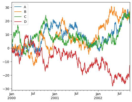
Nice to see we got a few things for “free”, like sane x-axis labels and the legend.

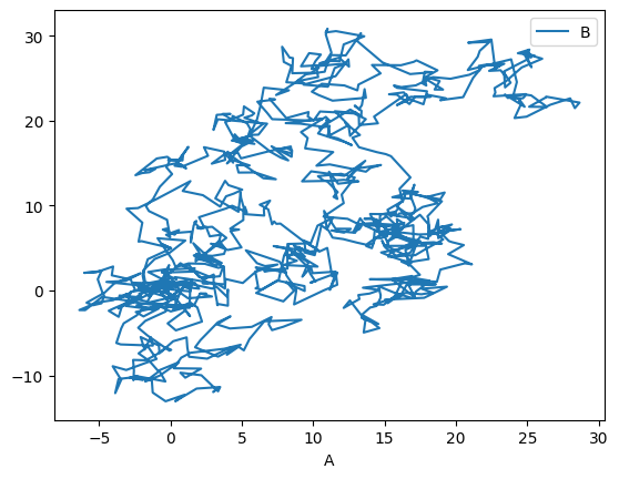
We can tell pandas which column corresponds to x, and which to y:

_ = df.plot(x='A', y='B')

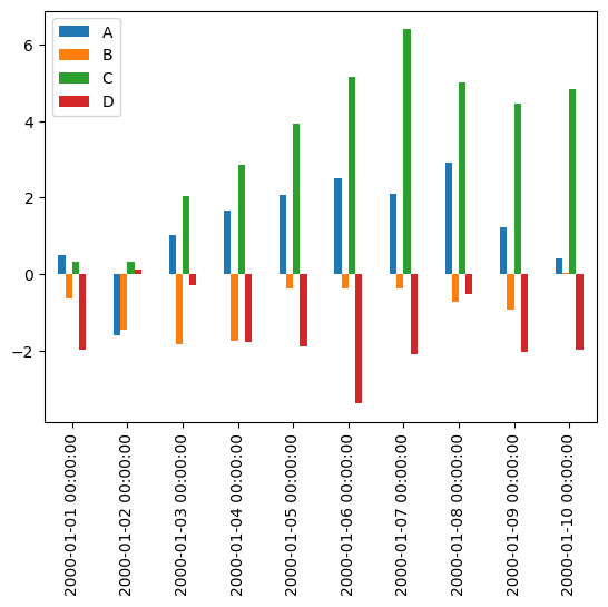
There are, of course, many possible types of plots that can be directly called from the pandas interface:

_ = df.iloc[:10, :].plot.bar()

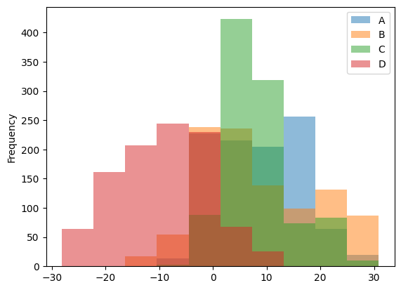
_ = df.plot.hist(alpha=0.5)

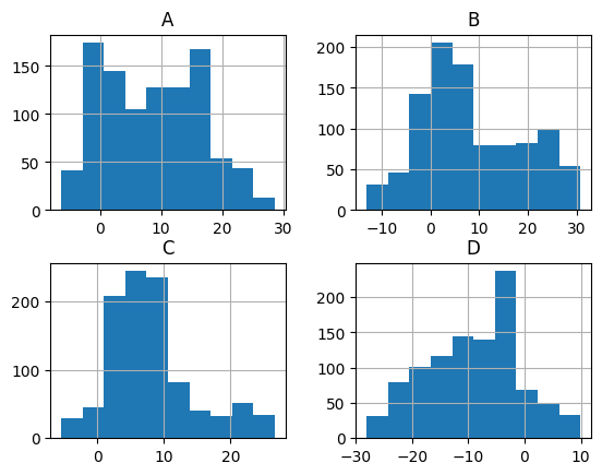
Histogramming each column separately can be done by calling the hist() method directly:

_ = df.hist()

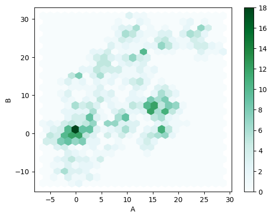
Lastly, a personal favorite:

_ = df.plot.hexbin(x='A', y='B', gridsize=25)

Altair

Matplotlib (and pandas’ interface to it) is the gold standard in the Python ecosystem - but there are other ecosystems as well. For example, vega-lite is a famous plotting library for the web and Javascript, and it uses a different grammar to define its plots. If you’re familiar with it you’ll be delighted to hear that Python’s altair provides bindings to it, and even if you’ve never heard of it it’s always nice to see that there are many other different ways to tell a computer how to draw stuff on the screen. Let’s look at a couple of examples:

import altair as alt

chart = alt.Chart(df)
chart.mark_point().encode(x='A', y='B')

In Altair you first create a chart object (a simple Chart above), and then you ask it to mark_point(), or mark_line(), to add that type of visualization to the chart. Then we specify the axis and other types of parameters (like color) and map (or encode) them to their corresponding column.

Let’s see how Altair works with other datatypes:

datetime_df = pd.DataFrame({'value': np.random.randn(100).cumsum()},
                           index=pd.date_range('2020', freq='D', periods=100))

datetime_df.head()

	value
2020-01-01	0.424336
2020-01-02	-0.765426
2020-01-03	-1.944647
2020-01-04	-0.561147
2020-01-05	-0.113494

chart = alt.Chart(datetime_df.reset_index())
chart.mark_line().encode(x='index:T', y='value:Q')

Above we plot the datetime data by telling Altair that the column named “index” is of type T, i.e. Time, while the column “value” is of type Q for quantitative.

One of the great things about these charts is that they can easily be made to be interactive:

from vega_datasets import data  # ready-made DFs for easy visualization examples

cars = data.cars
cars()

	Name	Miles_per_Gallon	Cylinders	Displacement	Horsepower	Weight_in_lbs	Acceleration	Year	Origin
0	chevrolet chevelle malibu	18.0	8	307.0	130.0	3504	12.0	1970-01-01	USA
1	buick skylark 320	15.0	8	350.0	165.0	3693	11.5	1970-01-01	USA
2	plymouth satellite	18.0	8	318.0	150.0	3436	11.0	1970-01-01	USA
3	amc rebel sst	16.0	8	304.0	150.0	3433	12.0	1970-01-01	USA
4	ford torino	17.0	8	302.0	140.0	3449	10.5	1970-01-01	USA
...	...	...	...	...	...	...	...	...	...
401	ford mustang gl	27.0	4	140.0	86.0	2790	15.6	1982-01-01	USA
402	vw pickup	44.0	4	97.0	52.0	2130	24.6	1982-01-01	Europe
403	dodge rampage	32.0	4	135.0	84.0	2295	11.6	1982-01-01	USA
404	ford ranger	28.0	4	120.0	79.0	2625	18.6	1982-01-01	USA
405	chevy s-10	31.0	4	119.0	82.0	2720	19.4	1982-01-01	USA

406 rows × 9 columns

cars_url = data.cars.url
cars_url  # The data is online and in json format which is standard practice for altair-based workflows

'https://cdn.jsdelivr.net/npm/vega-datasets@v1.29.0/data/cars.json'

alt.Chart(cars_url).mark_point().encode(
    x='Miles_per_Gallon:Q',
    y='Horsepower:Q',
    color='Origin:N',  # N for nominal, i.e. discrete and unordered (just like colors)
)

brush = alt.selection_interval()  # selection of type 'interval'

alt.Chart(cars_url).mark_point().encode(
    x='Miles_per_Gallon:Q',
    y='Horsepower:Q',
    color='Origin:N',  # N for nominal, i.e.discrete and unordered (just like colors)
).add_selection(brush)

The selection looks good but doesn’t do anything. Let’s add functionality:

alt.Chart(cars_url).mark_point().encode(
    x='Miles_per_Gallon:Q',
    y='Horsepower:Q',
    color=alt.condition(brush, 'Origin:N', alt.value('lightgray'))
).add_selection(
    brush
)

Altair has a ton more visualization types, some of which are more easily generated than others, and some are easier to generate using Altair rather than Matplotlib.

Bokeh, Holoviews and pandas-bokeh

Bokeh is another visualization effort in the Python ecosystem, but this time it revolves around web-based plots. Bokeh can be used directly, but it also serves as a backend plotting device for more advanced plotting libraries, like Holoviews and pandas-bokeh. It’s also designed in mind with huge datasets that don’t fit in memory, which is something that other tools might have trouble visualizing.

import bokeh
from bokeh.io import output_notebook, show
from bokeh.plotting import figure as bkfig
output_notebook()

Loading BokehJS ...

bokeh_figure = bkfig(width=400, height=400)
x = [1, 2, 3, 4, 5]
y = [6, 7, 2, 4, 5]
bokeh_figure.scatter(x,
                    y,
                    size=15,
                    line_color="navy",
                    fill_color="orange",
                    fill_alpha=0.5)

show(bokeh_figure)

We see how bokeh immediately outputs an interactive graph, i.e. an HTML document that will open in your browser (a couple of cells above we kindly asked bokeh to output its plots to the notebook instead). Bokeh can be used for many other types of plots, like:

datetime_df = datetime_df.reset_index()
datetime_df

	index	value
0	2020-01-01	0.424336
1	2020-01-02	-0.765426
2	2020-01-03	-1.944647
3	2020-01-04	-0.561147
4	2020-01-05	-0.113494
...	...	...
95	2020-04-05	-5.338371
96	2020-04-06	-6.155375
97	2020-04-07	-3.743377
98	2020-04-08	-4.073913
99	2020-04-09	-4.390383

100 rows × 2 columns

bokeh_figure_2 = bkfig(x_axis_type="datetime",
                       title="Value over Time",
                       height=350,
                       width=800)

bokeh_figure_2.xgrid.grid_line_color = None
bokeh_figure_2.ygrid.grid_line_alpha = 0.5
bokeh_figure_2.xaxis.axis_label = 'Time'
bokeh_figure_2.yaxis.axis_label = 'Value'

bokeh_figure_2.line(datetime_df.index, datetime_df.value)
show(bokeh_figure_2)

Let’s look at energy consumption, split by source (from the Pandas-Bokeh manual):

url = "https://raw.githubusercontent.com/PatrikHlobil/Pandas-Bokeh/master/docs/Testdata/energy/energy.csv"
df_energy = pd.read_csv(url, parse_dates=["Year"])
df_energy.head()

	Year	Oil	Gas	Coal	Nuclear Energy	Hydroelectricity	Other Renewable
0	1970-01-01	2291.5	826.7	1467.3	17.7	265.8	5.8
1	1971-01-01	2427.7	884.8	1459.2	24.9	276.4	6.3
2	1972-01-01	2613.9	933.7	1475.7	34.1	288.9	6.8
3	1973-01-01	2818.1	978.0	1519.6	45.9	292.5	7.3
4	1974-01-01	2777.3	1001.9	1520.9	59.6	321.1	7.7

Another Bokeh-based library is Holoviews. Its uniqueness stems from the way it handles DataFrames with multiple columns, and the way you add plots to each other. It’s very suitable for Jupyter notebook based plots:

import holoviews as hv
hv.extension("bokeh")

df_energy.head()

	Year	Oil	Gas	Coal	Nuclear Energy	Hydroelectricity	Other Renewable
0	1970-01-01	2291.5	826.7	1467.3	17.7	265.8	5.8
1	1971-01-01	2427.7	884.8	1459.2	24.9	276.4	6.3
2	1972-01-01	2613.9	933.7	1475.7	34.1	288.9	6.8
3	1973-01-01	2818.1	978.0	1519.6	45.9	292.5	7.3
4	1974-01-01	2777.3	1001.9	1520.9	59.6	321.1	7.7

scatter = hv.Scatter(df_energy, 'Oil', 'Gas')
scatter

scatter + hv.Curve(df_energy, 'Oil', 'Hydroelectricity')

def get_year_coal(df, year) -> int:
    return df.loc[df["Year"] == year, "Coal"]

items = {year: hv.Bars(get_year_coal(df_energy, year)) for year in df_energy["Year"]}
                       
hv.HoloMap(items, kdims=['Year'])

Holoviews really needs an entire class (or two) to go over its concepts, but once you get them you can create complicated visualizations which include a strong interactive component in a few lines of code.

Seaborn

A library which has really become a shining example of quick, efficient and clear plotting in the post-pandas era is seaborn. It combines many of the features of the previous libraries into a very concise API. Unlike a few of the previous libraries, however, it doesn’t use bokeh as its backend, but matplotlib, which means that the interactivity of the resulting plots isn’t as good. Be that as it may, it’s still a widely used library, and for good reasons.

In order to use seaborn to its full extent (and really all of the above libraries) we have to take a short detour and understand how to transform our data into a long-form format.

Once we have this long form data, we can put seaborn to the test.

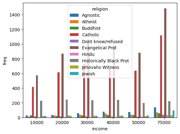
import seaborn as sns

income_barplot = sns.barplot(data=tidy_df, x='income', y='freq', hue='religion')

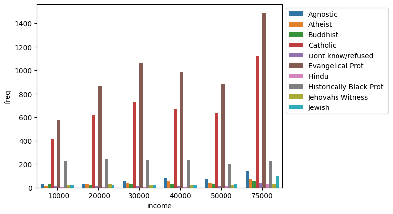
To fix the legend location:

income_barplot = sns.barplot(data=tidy_df, x='income', y='freq', hue='religion')
_ = income_barplot.legend(bbox_to_anchor=(1, 1))

Each seaborn visualization functions has a “data” keyword to which you pass your dataframe, and then a few other with which you specify the relations of the columns to one another. Look how simple it was to receive this beautiful bar chart.

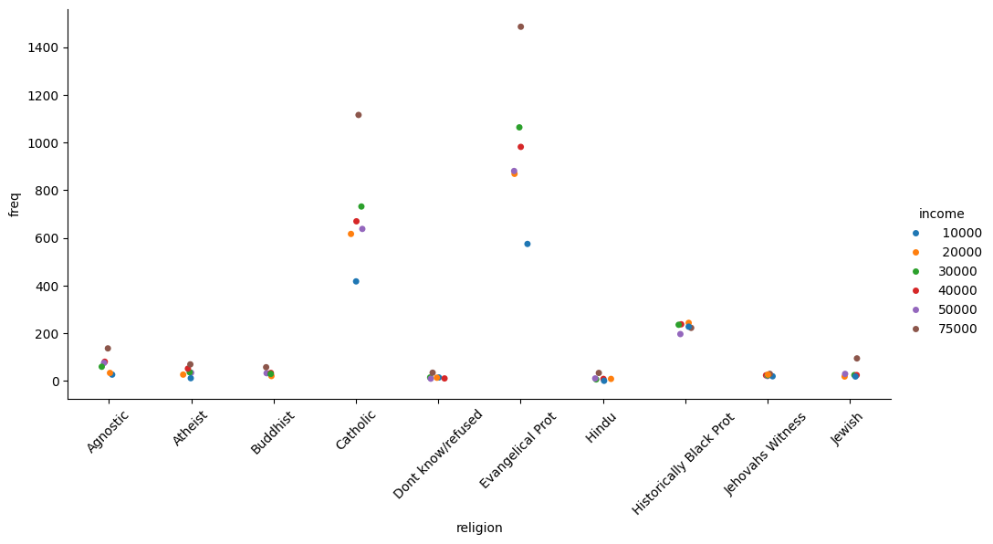
income_catplot = sns.catplot(data=tidy_df, x="religion", y="freq", hue="income", aspect=2)
_ = plt.xticks(rotation=45)

Seaborn also takes care of faceting the data for us:

_ = sns.catplot(data=tidy_df, x="religion", y="freq", hue="income", col="income")

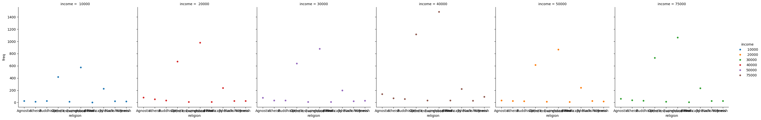
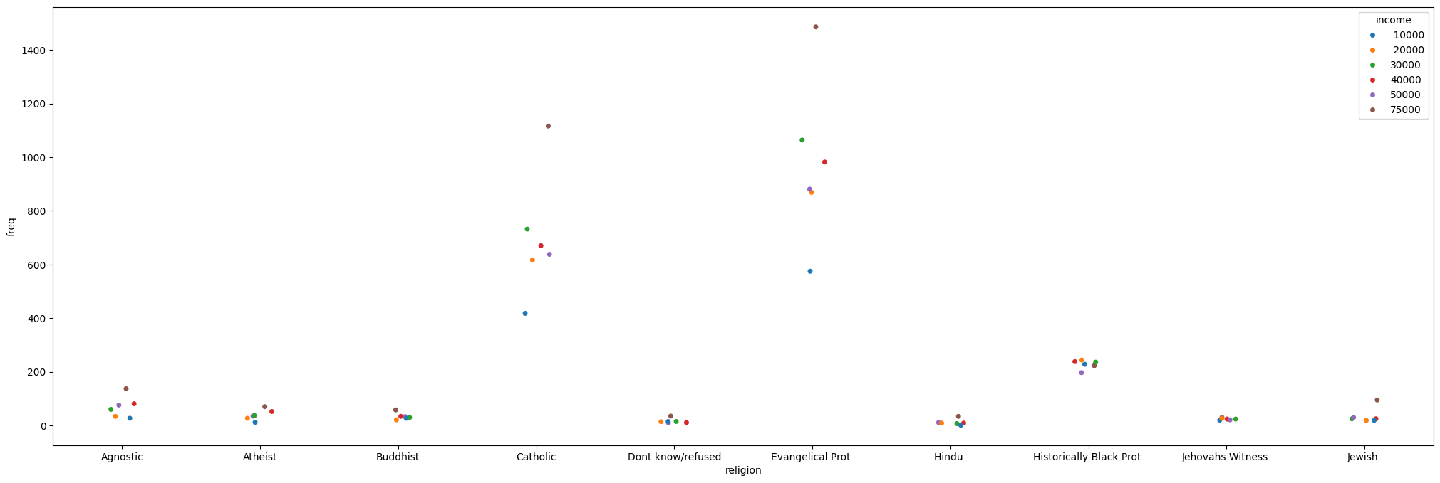
Figure is a bit small? We can use matplotlib to change it:

_, ax = plt.subplots(figsize=(25, 8))
_ = sns.stripplot(data=tidy_df, x="religion", y="freq", hue="income", ax=ax)

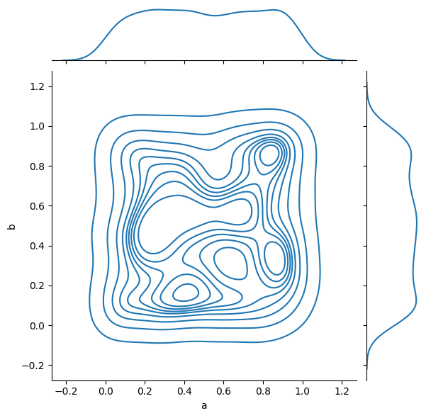
Simpler data can also be visualized, no need for categorical variables:

simple_df = pd.DataFrame(np.random.random((1000, 4)), columns=list('abcd'))
simple_df

	a	b	c	d
0	0.866067	0.496278	0.203062	0.400968
1	0.010828	0.999607	0.854796	0.232945
2	0.652564	0.647165	0.367135	0.474515
3	0.991972	0.889796	0.087627	0.168981
4	0.971222	0.692414	0.212155	0.929503
...	...	...	...	...
995	0.920265	0.162411	0.413716	0.025487
996	0.136229	0.752535	0.391649	0.320855
997	0.363096	0.666028	0.780295	0.086830
998	0.328681	0.587494	0.678299	0.702249
999	0.694159	0.672595	0.488958	0.942586

1000 rows × 4 columns

_ = sns.jointplot(data=simple_df, x='a', y='b', kind='kde')

And complex relations can also be visualized:

_ = sns.pairplot(data=simple_df)

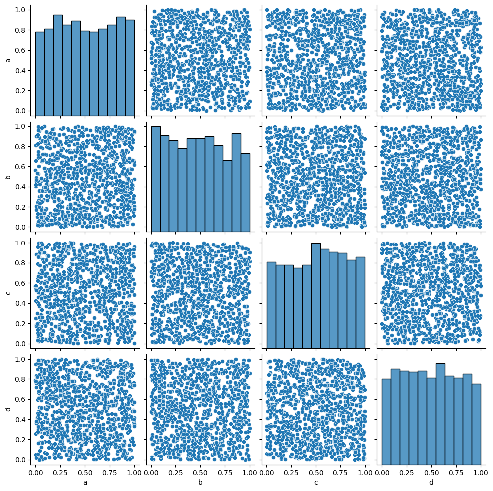
Seaborn should probably be your go-to choice when all you need is a 2D graph.

Higher Dimensionality: xarray

Pandas is amazing, but has its limits. A DataFrame can be a multi-dimensional container when using a MultiIndex, but it’s limited to a subset of uses in which another layer of indexing makes sense.

In many occasions, however, our data is truly high-dimensional. A simple case could be electro-physiological recordings, or calcium traces. In these cases we have several indices (some can be categorical), like “Sex”, “AnimalID”, “Date”, “TypeOfExperiment” and perhaps a few more. But the data itself is a vector of numbers representing voltage or fluorescence. Having this data in a dataframe seems a bit “off”, what are the columns on this dataframe? Is each column a voltage measurement? Or if each column is a measurement, how do you deal with the indices? We can use nested columns (MultiIndex the columns), but it’s not a very modular approach.

This is a classic example where pandas’ dataframes “fail”, and indeed pandas used to have a higher-dimensionality container named Panel. However, in late 2016 pandas developers deprecated it, publicly announcing that they intend to drop support for Panels sometime in the future, and whoever needs a higher-dimensionality container should use xarray.

xarray is a labeled n-dimensional array. Just like a DataFrame is a labeled 2D array, i.e. with names to its axes rather than numbers, in xarray each dimension has a name (time, temp, voltage) and its indices (“coordinates”) can also have labels (like a timestamp, for example). In addition, each xarray object also has metadata attached to it, in which we can write details that do not fit a columnar structure (experimenter name, hardware and software used for acquisition, etc.).

DataArray

import numpy as np
import xarray as xr

da = xr.DataArray(np.random.random((10, 2)))
da

<xarray.DataArray (dim_0: 10, dim_1: 2)> Size: 160B
array([[0.84316923, 0.45168906],
       [0.10629697, 0.36004292],
       [0.0574676 , 0.34534852],
       [0.9403532 , 0.09073964],
       [0.01857308, 0.33750266],
       [0.84216915, 0.76701275],
       [0.48395563, 0.20006189],
       [0.52264024, 0.58172156],
       [0.69518421, 0.88253301],
       [0.61616812, 0.83045222]])
Dimensions without coordinates: dim_0, dim_1

xarray.DataArray

• dim_0: 10
• dim_1: 2

• 0.8432 0.4517 0.1063 0.36 0.05747 ... 0.6952 0.8825 0.6162 0.8305

  array([[0.84316923, 0.45168906],
         [0.10629697, 0.36004292],
         [0.0574676 , 0.34534852],
         [0.9403532 , 0.09073964],
         [0.01857308, 0.33750266],
         [0.84216915, 0.76701275],
         [0.48395563, 0.20006189],
         [0.52264024, 0.58172156],
         [0.69518421, 0.88253301],
         [0.61616812, 0.83045222]])

• Coordinates: (0)
• Indexes: (0)
• Attributes: (0)

The basic building block of xarray is a DataArray, an n-dimensional counter part of a pandas’ Series. It has two dimensions, just like the numpy array that its based upon. We didn’t specify names for these dimensions, so currently they’re called dim_0 and dim_1. We also didn’t specify coordinates (indices), so the printout doesn’t report of any coordinates for the data.

da.values  # just like pandas

array([[0.84316923, 0.45168906],
       [0.10629697, 0.36004292],
       [0.0574676 , 0.34534852],
       [0.9403532 , 0.09073964],
       [0.01857308, 0.33750266],
       [0.84216915, 0.76701275],
       [0.48395563, 0.20006189],
       [0.52264024, 0.58172156],
       [0.69518421, 0.88253301],
       [0.61616812, 0.83045222]])

da.coords

Coordinates:
    *empty*

da.dims

('dim_0', 'dim_1')

da.attrs

{}

We’ll add coordinates and dimension names and see how indexing works:

dims = ('time', 'repetition')
coords = {'time': np.linspace(0, 1, num=10),
          'repetition': np.arange(2)}
da2 = xr.DataArray(np.random.random((10, 2)), dims=dims, coords=coords)
da2

<xarray.DataArray (time: 10, repetition: 2)> Size: 160B
array([[0.03592948, 0.95407936],
       [0.21129723, 0.68228822],
       [0.2013285 , 0.40468763],
       [0.58816598, 0.38706069],
       [0.26841336, 0.12459294],
       [0.14619846, 0.73606541],
       [0.98986978, 0.67060707],
       [0.70188417, 0.67591631],
       [0.82615898, 0.26929983],
       [0.80918357, 0.79687274]])
Coordinates:
  * time        (time) float64 80B 0.0 0.1111 0.2222 ... 0.7778 0.8889 1.0
  * repetition  (repetition) int64 16B 0 1

xarray.DataArray

• time: 10
• repetition: 2

• 0.03593 0.9541 0.2113 0.6823 0.2013 ... 0.8262 0.2693 0.8092 0.7969

  array([[0.03592948, 0.95407936],
         [0.21129723, 0.68228822],
         [0.2013285 , 0.40468763],
         [0.58816598, 0.38706069],
         [0.26841336, 0.12459294],
         [0.14619846, 0.73606541],
         [0.98986978, 0.67060707],
         [0.70188417, 0.67591631],
         [0.82615898, 0.26929983],
         [0.80918357, 0.79687274]])

• Coordinates: (2)
  • time
    (time)
    float64
    0.0 0.1111 0.2222 ... 0.8889 1.0

    array([0.      , 0.111111, 0.222222, 0.333333, 0.444444, 0.555556, 0.666667,
           0.777778, 0.888889, 1.      ])

  • repetition
    (repetition)
    int64
    0 1

    array([0, 1])

• Indexes: (2)
  • time
    PandasIndex

    PandasIndex(Index([               0.0, 0.1111111111111111, 0.2222222222222222,
           0.3333333333333333, 0.4444444444444444, 0.5555555555555556,
           0.6666666666666666, 0.7777777777777777, 0.8888888888888888,
                          1.0],
          dtype='float64', name='time'))

  • repetition
    PandasIndex

    PandasIndex(Index([0, 1], dtype='int64', name='repetition'))

• Attributes: (0)

da2.loc[0.1:0.3, 1]  # rows 1-2 in the second column

<xarray.DataArray (time: 2)> Size: 16B
array([0.68228822, 0.40468763])
Coordinates:
  * time        (time) float64 16B 0.1111 0.2222
    repetition  int64 8B 1

xarray.DataArray

• time: 2

• 0.6823 0.4047

  array([0.68228822, 0.40468763])

• Coordinates: (2)
  • time
    (time)
    float64
    0.1111 0.2222

    array([0.111111, 0.222222])

  • repetition
    ()
    int64
    1

    array(1)

• Indexes: (1)
  • time
    PandasIndex

    PandasIndex(Index([0.1111111111111111, 0.2222222222222222], dtype='float64', name='time'))

• Attributes: (0)

da2.isel(time=slice(3, 7))  # dimension name and integer label (sel = select)

<xarray.DataArray (time: 4, repetition: 2)> Size: 64B
array([[0.58816598, 0.38706069],
       [0.26841336, 0.12459294],
       [0.14619846, 0.73606541],
       [0.98986978, 0.67060707]])
Coordinates:
  * time        (time) float64 32B 0.3333 0.4444 0.5556 0.6667
  * repetition  (repetition) int64 16B 0 1

xarray.DataArray

• time: 4
• repetition: 2

• 0.5882 0.3871 0.2684 0.1246 0.1462 0.7361 0.9899 0.6706

  array([[0.58816598, 0.38706069],
         [0.26841336, 0.12459294],
         [0.14619846, 0.73606541],
         [0.98986978, 0.67060707]])

• Coordinates: (2)
  • time
    (time)
    float64
    0.3333 0.4444 0.5556 0.6667

    array([0.333333, 0.444444, 0.555556, 0.666667])

  • repetition
    (repetition)
    int64
    0 1

    array([0, 1])

• Indexes: (2)
  • time
    PandasIndex

    PandasIndex(Index([0.3333333333333333, 0.4444444444444444, 0.5555555555555556,
           0.6666666666666666],
          dtype='float64', name='time'))

  • repetition
    PandasIndex

    PandasIndex(Index([0, 1], dtype='int64', name='repetition'))

• Attributes: (0)

da2.sel(time=slice(0.1, 0.3), repetition=[1])  # dimension name and coordinate label

<xarray.DataArray (time: 2, repetition: 1)> Size: 16B
array([[0.68228822],
       [0.40468763]])
Coordinates:
  * time        (time) float64 16B 0.1111 0.2222
  * repetition  (repetition) int64 8B 1

xarray.DataArray

• time: 2
• repetition: 1

• 0.6823 0.4047

  array([[0.68228822],
         [0.40468763]])

• Coordinates: (2)
  • time
    (time)
    float64
    0.1111 0.2222

    array([0.111111, 0.222222])

  • repetition
    (repetition)
    int64
    1

    array([1])

• Indexes: (2)
  • time
    PandasIndex

    PandasIndex(Index([0.1111111111111111, 0.2222222222222222], dtype='float64', name='time'))

  • repetition
    PandasIndex

    PandasIndex(Index([1], dtype='int64', name='repetition'))

• Attributes: (0)

Other operations on DataArray instances, such as computations, grouping and such, are done very similarly to dataframes and numpy arrays.

Dataset

A Dataset is to a DataArray what a DataFrame is to a Series. In other words, it’s a collection of DataArray instances that share coordinates.

da2  # a reminder. We notice that this could've been a DataFrame as well

<xarray.DataArray (time: 10, repetition: 2)> Size: 160B
array([[0.03592948, 0.95407936],
       [0.21129723, 0.68228822],
       [0.2013285 , 0.40468763],
       [0.58816598, 0.38706069],
       [0.26841336, 0.12459294],
       [0.14619846, 0.73606541],
       [0.98986978, 0.67060707],
       [0.70188417, 0.67591631],
       [0.82615898, 0.26929983],
       [0.80918357, 0.79687274]])
Coordinates:
  * time        (time) float64 80B 0.0 0.1111 0.2222 ... 0.7778 0.8889 1.0
  * repetition  (repetition) int64 16B 0 1

xarray.DataArray

• time: 10
• repetition: 2

• 0.03593 0.9541 0.2113 0.6823 0.2013 ... 0.8262 0.2693 0.8092 0.7969

  array([[0.03592948, 0.95407936],
         [0.21129723, 0.68228822],
         [0.2013285 , 0.40468763],
         [0.58816598, 0.38706069],
         [0.26841336, 0.12459294],
         [0.14619846, 0.73606541],
         [0.98986978, 0.67060707],
         [0.70188417, 0.67591631],
         [0.82615898, 0.26929983],
         [0.80918357, 0.79687274]])

• Coordinates: (2)
  • time
    (time)
    float64
    0.0 0.1111 0.2222 ... 0.8889 1.0

    array([0.      , 0.111111, 0.222222, 0.333333, 0.444444, 0.555556, 0.666667,
           0.777778, 0.888889, 1.      ])

  • repetition
    (repetition)
    int64
    0 1

    array([0, 1])

• Indexes: (2)
  • time
    PandasIndex

    PandasIndex(Index([               0.0, 0.1111111111111111, 0.2222222222222222,
           0.3333333333333333, 0.4444444444444444, 0.5555555555555556,
           0.6666666666666666, 0.7777777777777777, 0.8888888888888888,
                          1.0],
          dtype='float64', name='time'))

  • repetition
    PandasIndex

    PandasIndex(Index([0, 1], dtype='int64', name='repetition'))

• Attributes: (0)

ds = xr.Dataset({'ephys': da2,
                 'calcium': ('time', np.random.random(10))},
                attrs={'AnimalD': 701,
                       'ExperimentType': 'double',
                       'Sex': 'Male'})
ds

<xarray.Dataset> Size: 336B
Dimensions:     (time: 10, repetition: 2)
Coordinates:
  * time        (time) float64 80B 0.0 0.1111 0.2222 ... 0.7778 0.8889 1.0
  * repetition  (repetition) int64 16B 0 1
Data variables:
    ephys       (time, repetition) float64 160B 0.03593 0.9541 ... 0.8092 0.7969
    calcium     (time) float64 80B 0.2909 0.03145 0.6968 ... 0.0332 0.4482
Attributes:
    AnimalD:         701
    ExperimentType:  double
    Sex:             Male

xarray.Dataset

• Dimensions:
  • time: 10
  • repetition: 2
• Coordinates: (2)
  • time
    (time)
    float64
    0.0 0.1111 0.2222 ... 0.8889 1.0

    array([0.      , 0.111111, 0.222222, 0.333333, 0.444444, 0.555556, 0.666667,
           0.777778, 0.888889, 1.      ])

  • repetition
    (repetition)
    int64
    0 1

    array([0, 1])

• Data variables: (2)
  • ephys
    (time, repetition)
    float64
    0.03593 0.9541 ... 0.8092 0.7969

    array([[0.03592948, 0.95407936],
           [0.21129723, 0.68228822],
           [0.2013285 , 0.40468763],
           [0.58816598, 0.38706069],
           [0.26841336, 0.12459294],
           [0.14619846, 0.73606541],
           [0.98986978, 0.67060707],
           [0.70188417, 0.67591631],
           [0.82615898, 0.26929983],
           [0.80918357, 0.79687274]])

  • calcium
    (time)
    float64
    0.2909 0.03145 ... 0.0332 0.4482

    array([0.29087884, 0.03144551, 0.69677575, 0.09198832, 0.81807385,
           0.66055174, 0.06729073, 0.74923504, 0.03320224, 0.44815079])

• Indexes: (2)
  • time
    PandasIndex

    PandasIndex(Index([               0.0, 0.1111111111111111, 0.2222222222222222,
           0.3333333333333333, 0.4444444444444444, 0.5555555555555556,
           0.6666666666666666, 0.7777777777777777, 0.8888888888888888,
                          1.0],
          dtype='float64', name='time'))

  • repetition
    PandasIndex

    PandasIndex(Index([0, 1], dtype='int64', name='repetition'))

• Attributes: (3)

  AnimalD :

  701

  ExperimentType :

  double

  Sex :

  Male

ds['ephys']  # individual DataArrays can be dissimilar in shape

<xarray.DataArray 'ephys' (time: 10, repetition: 2)> Size: 160B
array([[0.03592948, 0.95407936],
       [0.21129723, 0.68228822],
       [0.2013285 , 0.40468763],
       [0.58816598, 0.38706069],
       [0.26841336, 0.12459294],
       [0.14619846, 0.73606541],
       [0.98986978, 0.67060707],
       [0.70188417, 0.67591631],
       [0.82615898, 0.26929983],
       [0.80918357, 0.79687274]])
Coordinates:
  * time        (time) float64 80B 0.0 0.1111 0.2222 ... 0.7778 0.8889 1.0
  * repetition  (repetition) int64 16B 0 1

xarray.DataArray

'ephys'

• time: 10
• repetition: 2

• 0.03593 0.9541 0.2113 0.6823 0.2013 ... 0.8262 0.2693 0.8092 0.7969

  array([[0.03592948, 0.95407936],
         [0.21129723, 0.68228822],
         [0.2013285 , 0.40468763],
         [0.58816598, 0.38706069],
         [0.26841336, 0.12459294],
         [0.14619846, 0.73606541],
         [0.98986978, 0.67060707],
         [0.70188417, 0.67591631],
         [0.82615898, 0.26929983],
         [0.80918357, 0.79687274]])

• Coordinates: (2)
  • time
    (time)
    float64
    0.0 0.1111 0.2222 ... 0.8889 1.0

    array([0.      , 0.111111, 0.222222, 0.333333, 0.444444, 0.555556, 0.666667,
           0.777778, 0.888889, 1.      ])

  • repetition
    (repetition)
    int64
    0 1

    array([0, 1])

• Indexes: (2)
  • time
    PandasIndex

    PandasIndex(Index([               0.0, 0.1111111111111111, 0.2222222222222222,
           0.3333333333333333, 0.4444444444444444, 0.5555555555555556,
           0.6666666666666666, 0.7777777777777777, 0.8888888888888888,
                          1.0],
          dtype='float64', name='time'))

  • repetition
    PandasIndex

    PandasIndex(Index([0, 1], dtype='int64', name='repetition'))

• Attributes: (0)

Exercise: Rat Visual Stimulus Experiment Database

You’re measuring the potential of neurons in a rat’s brain over time in response to flashes of light using a multi-electrode array surgically inserted into the rat’s skull. Each trial is two seconds long, and one second into the trial a short, 100 ms, bright light is flashed at the animal. After 30 seconds the experiment is replicated, for a total of 4 repetitions. The relevant parameters are the following:

• Rat ID.

• Experimenter name.

• Rat gender.

• Measured voltage (10 electrode, 10k samples representing two seconds).

• Stimulus index (mark differently the pre-, during- and post-stimulus time).

• Repetition number.

Mock data and model it, you can add more parameters if you feel so.

Experimental timeline:

       1s          100ms             0.9s             30s
Start -----> Flash -----> End flash -----> End trial -----> New trial
|                                                                    |
|--------------------------------------------------------------------|
                                   x4

Methods and functions to implement

1. There should be a class holding this data table, VisualStimData, alongside several methods for the analysis of the data. The class should have a data attribute containing the data table, in a xarray.DataArray or a xarray.Dataset.

2. Write a function (not a method) that returns an instance of the class with mock data.

   def mock_stim_data() -> VisualStimData:
       """ Creates a new VisualStimData instance with mock data """
   

   When simulating the recorded voltage, it’s completely fine to not model spikes precisely, with leaky integration and so forth - randoming numbers and treating them as the recorded neural potential is fine. There are quite a few ways to model real neurons, if so you wish, brian being one of them. If your own research will benefit from knowing how to use these tools, this exercise is a great place to start familiarizing yourself with them.

3. Write a method that receives a repetition number, rat ID, and a list of electrode numbers, and plots the voltage recorded from these electrodes. The single figure should be divided into however many plots needed, depending on the length of the list of electrode numbers.

   def plot_electrode(self, rep_number: int, rat_id: int, elec_number: tuple=(0,)):
       """
       Plots the voltage of the electrodes in "elec_number" for the rat "rat_id" in the repetition
       "rep_number". Shows a single figure with subplots.
       """
   

4. To see if the different experimenters influence the measurements, write a method that calculates the mean, standard deviation and median of the average voltage trace across all repetitions, for each experimenter, and shows a bar plot of it.

   def experimenter_bias(self):
       """ Shows the statistics of the average recording across all experimenters """
   

Exercise solutions below…

Show code cell source Hide code cell source

import xarray as xr
import numpy as np
import pandas as pd
import matplotlib.pyplot as plt


class VisualStimData:
    """
    Data and methods for the visual stimulus ePhys experiment.
    The data table itself is held in self.data, an `xarray` object.
    Inputs:
        data: xr.DataArray or xr.Dataset
    Methods:
         ...
    """
    def __init__(self, data: xr.Dataset, ):
        assert isinstance(data, xr.Dataset)
        self.data = data


    def plot_electrode(self, rep_number: int, rat_id: int, elec_number: tuple=(0,)):
        """
        Plots the voltage of the electrodes in "elec_number" for the rat "rat_id" in the repetition
        "rep_number". Shows a single figure with two subplots, for male and female rats.
        """
        fig, axes = plt.subplots(len(elec_number), 1)
        axes = np.array([axes]) if isinstance(axes, plt.Axes) else axes
        time = self.data['time']
        for ax, elec in zip(axes, elec_number):
            to_plot = self.data.sel(rep=rep_number, rat_id=rat_id, elec=elec)['volt'].values
            ax.plot(time, to_plot)
            ax.set_xlabel('Time [s]')
            ax.set_ylabel('Voltage [V]')
            ax.set_title(f'Electrode {elec}')

        fig.tight_layout()

    def experimenter_bias(self):
        """ Shows the statistics of the average recording across all experimenters """
        names = np.unique(self.data.coords['exp_name'].values)
        means = []
        stds = []
        medians = []
        for experimenter in names:
            data = self.data.sel(exp_name=experimenter)['volt'].values
            means.append(np.abs(data.mean()))
            stds.append(np.abs(data.std()))
            medians.append(np.abs(np.median(data)))

        # Plotting
        fig, ax = plt.subplots()
        x_locs = np.arange(len(names))
        width = 0.3
        rect0 = ax.bar(x_locs, means, width, color='C0')
        rect1 = ax.bar(x_locs + width, stds, width, color='C1')
        rect2 = ax.bar(x_locs - width, medians, width, color='C2')

        ax.set_xticks(x_locs)
        ax.set_xticklabels(names)
        ax.legend((rect0[0], rect1[0], rect2[0]), ('Mean', 'STD', 'Median'))
        ax.set_title('Experimenter Bias (absolute values)')
        ax.set_ylabel('Volts [V]')

Show code cell source Hide code cell source

def mock_stim_data() -> VisualStimData:
    """ Creates a new VisualStimData instance with mock data """
    num_of_animals = 20
    num_of_reps = 4
    reps = np.arange(num_of_reps, dtype=np.uint8)
    total_num_of_exp = num_of_animals * num_of_reps
    exp_number = np.arange(total_num_of_exp, dtype=np.uint32)
    
    rat_id_ints, rat_id = _generate_rat_data(num_of_animals)
    room_temp, room_humid = _generate_temp_hum_values(total_num_of_exp)
    experimenters = _generate_experimenter_names(num_of_animals, num_of_reps)
    rat_sex = _generate_rat_gender(num_of_animals, num_of_reps)
    stim, electrode_array, time, volt = _generate_voltage_stim(num_of_animals, num_of_reps)

    # Construct the Dataset - this could be done with a pd.MultiIndex as well
    ds = xr.Dataset({'temp': (['num'], room_temp),
                     'humid': (['num'], room_humid),
                     'volt': (['elec', 'time', 'rat_id', 'rep'], volt),
                     'stim': (['time'], stim)},
                    coords={'elec': electrode_array,
                            'time': time,
                            'rat_id': rat_id,
                            'rep': reps,
                            'exp_name': experimenters,
                            'sex': rat_sex,
                            'num': exp_number,
                            })

    ds.attrs['exp_date'] = pd.to_datetime('today')
    ds.attrs['rat_strain'] = 'Sprague Dawley'

    return VisualStimData(ds)
    
def _generate_rat_data(num_of_animals):
    rat_id_ints = np.random.choice(np.arange(100, 900), size=300, replace=False)
    rat_id = np.random.choice(rat_id_ints, size=num_of_animals, replace=False)
    return rat_id_ints, rat_id


def _generate_temp_hum_values(total_num_of_exp):
    room_temp = np.random.random(total_num_of_exp) * 3 + 23  # between 23 and 26 C
    room_humid = np.random.randint(30, 70, size=total_num_of_exp)
    return room_temp, room_humid

def _generate_experimenter_names(num_of_animals, num_of_reps):
    names = ['Dana', 'Motti', 'Sam', 'Daria']
    experimenters = np.random.choice(names, size=num_of_animals, replace=True)
    experimenters = np.tile(experimenters, num_of_reps)
    return experimenters

def _generate_rat_gender(num_of_animals, num_of_reps):
    sex = ['F', 'M']
    rat_sex = np.random.choice(sex, size=num_of_animals, replace=True)
    rat_sex = np.tile(rat_sex, num_of_reps)
    return rat_sex


def _generate_voltage_stim(num_of_animals, num_of_reps):
    pre_stim = 1  # seconds
    stim_time = 0.1  # seconds
    post_stim = 0.9  # seconds
    sampling_rate = 5000  # Hz
    freq = 1 / sampling_rate
    experiment_length = int(pre_stim + stim_time + post_stim)
    electrodes = 10
    samples = sampling_rate * experiment_length

    # Random voltage values from N(0.068, 0.0004)
    volt = 0.02 * np.random.randn(electrodes, samples, num_of_animals,
                                 num_of_reps).astype(np.float32) - 0.068  # in volts, not millivolts
    volt[volt > -0.02] = 0.04  # "spikes"
    time = pd.date_range(start=pd.to_datetime('today'), periods=experiment_length * sampling_rate,
                         freq=f'{freq}S')
    electrode_array = np.arange(electrodes, dtype=np.uint16)

    # Stim index - -1 is pre, 0 is stim, 1 is post
    stim = np.zeros(int(samples), dtype=np.int8)
    stim[:int(pre_stim*sampling_rate)] = -1
    stim[int((pre_stim + stim_time)*sampling_rate):] += 1
    return stim, electrode_array, time, volt

Show code cell source Hide code cell source

# Run the solution
stim_data = mock_stim_data()
ids = stim_data.data['rat_id']
arr = stim_data.plot_electrode(rep_number=2, rat_id=ids[0], elec_number=(1, 6))
stim_data.experimenter_bias()

/tmp/ipykernel_2203/2117857072.py:72: FutureWarning: 'S' is deprecated and will be removed in a future version, please use 's' instead.
  time = pd.date_range(start=pd.to_datetime('today'), periods=experiment_length * sampling_rate,

Show code cell source Hide code cell source

stim_data.data

<xarray.Dataset> Size: 32MB
Dimensions:   (num: 80, elec: 10, time: 10000, rat_id: 20, rep: 4,
               exp_name: 80, sex: 80)
Coordinates:
  * elec      (elec) uint16 20B 0 1 2 3 4 5 6 7 8 9
  * time      (time) datetime64[ns] 80kB 2025-05-12T07:52:01.258663 ... 2025-...
  * rat_id    (rat_id) int64 160B 185 875 136 322 810 ... 804 847 269 516 111
  * rep       (rep) uint8 4B 0 1 2 3
  * exp_name  (exp_name) <U5 2kB 'Daria' 'Motti' 'Dana' ... 'Motti' 'Dana'
  * sex       (sex) <U1 320B 'M' 'M' 'M' 'M' 'M' 'M' ... 'M' 'F' 'M' 'M' 'F' 'M'
  * num       (num) uint32 320B 0 1 2 3 4 5 6 7 8 ... 71 72 73 74 75 76 77 78 79
Data variables:
    temp      (num) float64 640B 25.9 23.8 23.23 23.76 ... 23.36 24.86 25.28
    humid     (num) int64 640B 40 40 62 59 49 64 64 59 ... 33 57 37 50 47 47 40
    volt      (elec, time, rat_id, rep) float32 32MB -0.09001 ... -0.07046
    stim      (time) int8 10kB -1 -1 -1 -1 -1 -1 -1 -1 -1 ... 1 1 1 1 1 1 1 1 1
Attributes:
    exp_date:    2025-05-12 07:52:01.261832
    rat_strain:  Sprague Dawley

xarray.Dataset

• Dimensions:
  • num: 80
  • elec: 10
  • time: 10000
  • rat_id: 20
  • rep: 4
  • exp_name: 80
  • sex: 80
• Coordinates: (7)
  • elec
    (elec)
    uint16
    0 1 2 3 4 5 6 7 8 9

    array([0, 1, 2, 3, 4, 5, 6, 7, 8, 9], dtype=uint16)

  • time
    (time)
    datetime64[ns]
    2025-05-12T07:52:01.258663 ... 2...

    array(['2025-05-12T07:52:01.258663000', '2025-05-12T07:52:01.258863000',
           '2025-05-12T07:52:01.259063000', ..., '2025-05-12T07:52:03.258063000',
           '2025-05-12T07:52:03.258263000', '2025-05-12T07:52:03.258463000'],
          shape=(10000,), dtype='datetime64[ns]')

  • rat_id
    (rat_id)
    int64
    185 875 136 322 ... 847 269 516 111

    array([185, 875, 136, 322, 810, 371, 478, 159, 209, 512, 503, 328, 301, 439,
           133, 804, 847, 269, 516, 111])

  • rep
    (rep)
    uint8
    0 1 2 3

    array([0, 1, 2, 3], dtype=uint8)

  • exp_name
    (exp_name)
    <U5
    'Daria' 'Motti' ... 'Motti' 'Dana'

    array(['Daria', 'Motti', 'Dana', 'Motti', 'Motti', 'Dana', 'Dana', 'Sam',
           'Dana', 'Motti', 'Daria', 'Daria', 'Dana', 'Daria', 'Daria', 'Sam',
           'Motti', 'Daria', 'Motti', 'Dana', 'Daria', 'Motti', 'Dana', 'Motti',
           'Motti', 'Dana', 'Dana', 'Sam', 'Dana', 'Motti', 'Daria', 'Daria',
           'Dana', 'Daria', 'Daria', 'Sam', 'Motti', 'Daria', 'Motti', 'Dana',
           'Daria', 'Motti', 'Dana', 'Motti', 'Motti', 'Dana', 'Dana', 'Sam',
           'Dana', 'Motti', 'Daria', 'Daria', 'Dana', 'Daria', 'Daria', 'Sam',
           'Motti', 'Daria', 'Motti', 'Dana', 'Daria', 'Motti', 'Dana', 'Motti',
           'Motti', 'Dana', 'Dana', 'Sam', 'Dana', 'Motti', 'Daria', 'Daria',
           'Dana', 'Daria', 'Daria', 'Sam', 'Motti', 'Daria', 'Motti', 'Dana'],
          dtype='<U5')

  • sex
    (sex)
    <U1
    'M' 'M' 'M' 'M' ... 'M' 'M' 'F' 'M'

    array(['M', 'M', 'M', 'M', 'M', 'M', 'M', 'F', 'M', 'F', 'F', 'M', 'M', 'F',
           'M', 'F', 'M', 'M', 'F', 'M', 'M', 'M', 'M', 'M', 'M', 'M', 'M', 'F',
           'M', 'F', 'F', 'M', 'M', 'F', 'M', 'F', 'M', 'M', 'F', 'M', 'M', 'M',
           'M', 'M', 'M', 'M', 'M', 'F', 'M', 'F', 'F', 'M', 'M', 'F', 'M', 'F',
           'M', 'M', 'F', 'M', 'M', 'M', 'M', 'M', 'M', 'M', 'M', 'F', 'M', 'F',
           'F', 'M', 'M', 'F', 'M', 'F', 'M', 'M', 'F', 'M'], dtype='<U1')

  • num
    (num)
    uint32
    0 1 2 3 4 5 6 ... 74 75 76 77 78 79

    array([ 0,  1,  2,  3,  4,  5,  6,  7,  8,  9, 10, 11, 12, 13, 14, 15, 16, 17,
           18, 19, 20, 21, 22, 23, 24, 25, 26, 27, 28, 29, 30, 31, 32, 33, 34, 35,
           36, 37, 38, 39, 40, 41, 42, 43, 44, 45, 46, 47, 48, 49, 50, 51, 52, 53,
           54, 55, 56, 57, 58, 59, 60, 61, 62, 63, 64, 65, 66, 67, 68, 69, 70, 71,
           72, 73, 74, 75, 76, 77, 78, 79], dtype=uint32)

• Data variables: (4)
  • temp
    (num)
    float64
    25.9 23.8 23.23 ... 24.86 25.28

    array([25.89554034, 23.80471268, 23.2330364 , 23.75709082, 24.27857109,
           23.40164026, 23.63651629, 25.74810441, 25.79629319, 25.45661092,
           23.33886832, 23.23529711, 25.50887424, 23.86616661, 24.06046401,
           25.29735611, 24.52549966, 24.78731601, 25.27712179, 23.4121459 ,
           23.53197038, 25.69447658, 23.87641626, 25.43797979, 24.60367221,
           25.55701919, 23.246351  , 24.29897247, 24.65636573, 23.79213806,
           25.14159824, 24.94453502, 25.66191508, 24.09929995, 23.05459308,
           25.40095481, 25.23260064, 23.7664687 , 25.48506096, 23.21543967,
           25.16902368, 23.80307583, 23.94319328, 23.48090916, 23.83599325,
           24.84578966, 24.81992667, 25.88757372, 25.57616725, 25.25121188,
           25.33629956, 25.58158226, 25.80292436, 25.27599654, 23.46889988,
           24.64416641, 25.40646901, 24.62903896, 24.12778529, 23.48913771,
           25.31579986, 24.73934594, 25.39012009, 25.84633426, 24.42101296,
           25.01929768, 25.56108311, 24.95667898, 24.9649958 , 25.19870588,
           25.98690191, 23.89629663, 23.38171525, 24.12751895, 24.52497186,
           25.66357721, 23.18161789, 23.35577664, 24.85744255, 25.27960792])

  • humid
    (num)
    int64
    40 40 62 59 49 ... 37 50 47 47 40

    array([40, 40, 62, 59, 49, 64, 64, 59, 57, 39, 36, 69, 68, 68, 68, 43, 62,
           55, 40, 51, 51, 43, 50, 34, 52, 69, 35, 36, 30, 33, 61, 38, 49, 53,
           37, 64, 35, 31, 55, 41, 48, 36, 38, 69, 65, 53, 50, 56, 42, 32, 33,
           35, 42, 69, 52, 54, 40, 66, 43, 67, 60, 68, 33, 58, 65, 37, 31, 54,
           63, 46, 41, 33, 30, 33, 57, 37, 50, 47, 47, 40])

  • volt
    (elec, time, rat_id, rep)
    float32
    -0.09001 -0.03466 ... -0.07046

    array([[[[-0.09000953, -0.0346598 , -0.05877034, -0.06151881],
             [-0.07675636, -0.07209603, -0.08324058, -0.06509262],
             [-0.08352926, -0.09371206, -0.10080995, -0.08550729],
             ...,
             [-0.10234061, -0.05741658, -0.06725498, -0.1006574 ],
             [-0.07922129, -0.0289382 , -0.05921644, -0.09082416],
             [-0.08322541, -0.05502279, -0.05238608, -0.06721566]],
    
            [[-0.07686982, -0.07864012, -0.09993018, -0.09354296],
             [-0.05516525, -0.08964665, -0.08793139, -0.03301274],
             [-0.06040586, -0.05448773, -0.1129723 , -0.0774111 ],
             ...,
             [-0.08411969, -0.02647552, -0.06027994, -0.04827461],
             [-0.07398934, -0.07834311, -0.06201305, -0.09011085],
             [-0.04527374, -0.05386845, -0.06100827, -0.08436842]],
    
            [[-0.06036105, -0.0866407 , -0.07321113, -0.05033187],
             [-0.06091734, -0.09157221, -0.06922716, -0.07310615],
             [-0.08604217, -0.03638666, -0.05042487, -0.10626291],
             ...,
    ...
             [-0.06748295, -0.03638955, -0.05093579, -0.10742304],
             [-0.08746907, -0.06495476, -0.02584663, -0.06592189],
             [-0.09318155, -0.07544124, -0.08018081, -0.06873948]],
    
            [[-0.06104205, -0.07560357, -0.06678611, -0.06827927],
             [-0.06764179, -0.04905694, -0.09761745, -0.06798726],
             [-0.06316345, -0.02478241, -0.09672603, -0.09160584],
             ...,
             [-0.07074688, -0.05267135, -0.06835388, -0.05997064],
             [-0.06195877,  0.04      , -0.03135167, -0.05570206],
             [-0.08491243, -0.05390181, -0.04352784, -0.09346013]],
    
            [[-0.092477  , -0.05850282, -0.04495519, -0.04319137],
             [-0.05001903, -0.0626077 , -0.0927373 , -0.05791388],
             [-0.06172635, -0.09005577, -0.06898838, -0.0724382 ],
             ...,
             [-0.02927185, -0.0436735 , -0.05946907,  0.04      ],
             [-0.04720864, -0.0441069 , -0.07003775, -0.07115723],
             [-0.03522818, -0.05186625, -0.07198861, -0.07045846]]]],
          shape=(10, 10000, 20, 4), dtype=float32)

  • stim
    (time)
    int8
    -1 -1 -1 -1 -1 -1 ... 1 1 1 1 1 1

    array([-1, -1, -1, ...,  1,  1,  1], shape=(10000,), dtype=int8)

• Indexes: (7)
  • elec
    PandasIndex

    PandasIndex(Index([0, 1, 2, 3, 4, 5, 6, 7, 8, 9], dtype='uint16', name='elec'))

  • time
    PandasIndex

    PandasIndex(DatetimeIndex(['2025-05-12 07:52:01.258663', '2025-05-12 07:52:01.258863',
                   '2025-05-12 07:52:01.259063', '2025-05-12 07:52:01.259263',
                   '2025-05-12 07:52:01.259463', '2025-05-12 07:52:01.259663',
                   '2025-05-12 07:52:01.259863', '2025-05-12 07:52:01.260063',
                   '2025-05-12 07:52:01.260263', '2025-05-12 07:52:01.260463',
                   ...
                   '2025-05-12 07:52:03.256663', '2025-05-12 07:52:03.256863',
                   '2025-05-12 07:52:03.257063', '2025-05-12 07:52:03.257263',
                   '2025-05-12 07:52:03.257463', '2025-05-12 07:52:03.257663',
                   '2025-05-12 07:52:03.257863', '2025-05-12 07:52:03.258063',
                   '2025-05-12 07:52:03.258263', '2025-05-12 07:52:03.258463'],
                  dtype='datetime64[ns]', name='time', length=10000, freq='200us'))

  • rat_id
    PandasIndex

    PandasIndex(Index([185, 875, 136, 322, 810, 371, 478, 159, 209, 512, 503, 328, 301, 439,
           133, 804, 847, 269, 516, 111],
          dtype='int64', name='rat_id'))

  • rep
    PandasIndex

    PandasIndex(Index([0, 1, 2, 3], dtype='uint8', name='rep'))

  • exp_name
    PandasIndex

    PandasIndex(Index(['Daria', 'Motti', 'Dana', 'Motti', 'Motti', 'Dana', 'Dana', 'Sam',
           'Dana', 'Motti', 'Daria', 'Daria', 'Dana', 'Daria', 'Daria', 'Sam',
           'Motti', 'Daria', 'Motti', 'Dana', 'Daria', 'Motti', 'Dana', 'Motti',
           'Motti', 'Dana', 'Dana', 'Sam', 'Dana', 'Motti', 'Daria', 'Daria',
           'Dana', 'Daria', 'Daria', 'Sam', 'Motti', 'Daria', 'Motti', 'Dana',
           'Daria', 'Motti', 'Dana', 'Motti', 'Motti', 'Dana', 'Dana', 'Sam',
           'Dana', 'Motti', 'Daria', 'Daria', 'Dana', 'Daria', 'Daria', 'Sam',
           'Motti', 'Daria', 'Motti', 'Dana', 'Daria', 'Motti', 'Dana', 'Motti',
           'Motti', 'Dana', 'Dana', 'Sam', 'Dana', 'Motti', 'Daria', 'Daria',
           'Dana', 'Daria', 'Daria', 'Sam', 'Motti', 'Daria', 'Motti', 'Dana'],
          dtype='object', name='exp_name'))

  • sex
    PandasIndex

    PandasIndex(Index(['M', 'M', 'M', 'M', 'M', 'M', 'M', 'F', 'M', 'F', 'F', 'M', 'M', 'F',
           'M', 'F', 'M', 'M', 'F', 'M', 'M', 'M', 'M', 'M', 'M', 'M', 'M', 'F',
           'M', 'F', 'F', 'M', 'M', 'F', 'M', 'F', 'M', 'M', 'F', 'M', 'M', 'M',
           'M', 'M', 'M', 'M', 'M', 'F', 'M', 'F', 'F', 'M', 'M', 'F', 'M', 'F',
           'M', 'M', 'F', 'M', 'M', 'M', 'M', 'M', 'M', 'M', 'M', 'F', 'M', 'F',
           'F', 'M', 'M', 'F', 'M', 'F', 'M', 'M', 'F', 'M'],
          dtype='object', name='sex'))

  • num
    PandasIndex

    PandasIndex(Index([ 0,  1,  2,  3,  4,  5,  6,  7,  8,  9, 10, 11, 12, 13, 14, 15, 16, 17,
           18, 19, 20, 21, 22, 23, 24, 25, 26, 27, 28, 29, 30, 31, 32, 33, 34, 35,
           36, 37, 38, 39, 40, 41, 42, 43, 44, 45, 46, 47, 48, 49, 50, 51, 52, 53,
           54, 55, 56, 57, 58, 59, 60, 61, 62, 63, 64, 65, 66, 67, 68, 69, 70, 71,
           72, 73, 74, 75, 76, 77, 78, 79],
          dtype='uint32', name='num'))

• Attributes: (2)

  exp_date :

  2025-05-12 07:52:01.261832

  rat_strain :

  Sprague Dawley