Class 7a: More pandas#
More pandas!#
Working with String DataFrames#
Pandas’ Series instances with a dtype of object or string expose a str attribute that enables vectorized string operations. These can come in tremendously handy, particularly when cleaning the data and performing aggregations on manually submitted fields.
Let’s imagine having the misfortune of reading some CSV data and finding the following headers:
import pandas as pd
import numpy as np
import matplotlib.pyplot as plt

messy_strings = [
    'Id___name', 'AGE', ' DomHand ', np.nan, 'qid    score1', 'score2', 3,
    ' COLOR_ SHAPe   _size', 'origin_residence immigration'
]
s = pd.Series(messy_strings, dtype="string", name="Messy Strings")
s
0                       Id___name
1                             AGE
2                        DomHand
3                            <NA>
4                   qid    score1
5                          score2
6                               3
7            COLOR_ SHAPe   _size
8    origin_residence immigration
Name: Messy Strings, dtype: string
To try and parse something more reasonable, we might first want to remove all unnecessary whitespace and underscores. One way to achieve that would be:
s_1 = s.str.strip().str.replace("[_\s]+", " ", regex=True).str.lower()
s_1
0                         id name
1                             age
2                         domhand
3                            <NA>
4                      qid score1
5                          score2
6                               3
7                color shape size
8    origin residence immigration
Name: Messy Strings, dtype: string
Let’s break this down:
strip()removed all whitespace from the beginning and end of the string.We used a regular expression to replace all one or more (
+) occurrences of whitespace (\s) and underscores with single spaces.We converted all characters to lowercase.
Next, we’ll split() strings separated by whitespace and extract an array of the values:
s_2 = s_1.str.split(expand=True)
print(f"DataFrame:\n{s_2}")

s_3 = s_2.to_numpy().flatten()
print(f"\nArray:\n{s_3}")
DataFrame:
         0          1            2
0       id       name         <NA>
1      age       <NA>         <NA>
2  domhand       <NA>         <NA>
3     <NA>       <NA>         <NA>
4      qid     score1         <NA>
5   score2       <NA>         <NA>
6        3       <NA>         <NA>
7    color      shape         size
8   origin  residence  immigration

Array:
['id' 'name' <NA> 'age' <NA> <NA> 'domhand' <NA> <NA> <NA> <NA> <NA> 'qid'
 'score1' <NA> 'score2' <NA> <NA> '3' <NA> <NA> 'color' 'shape' 'size'
 'origin' 'residence' 'immigration']
Finally, we can get rid of the <NA> values:
column_names = s_3[~pd.isnull(s_3)]
column_names
array(['id', 'name', 'age', 'domhand', 'qid', 'score1', 'score2', '3',
       'color', 'shape', 'size', 'origin', 'residence', 'immigration'],
      dtype=object)
DataFrame String Operations Exercise
Generate a 1000x1 shaped
pd.DataFramefilled with 3-letter strings. Use thestringmodule’sascii_lowercaseattribute and numpy’srandommodule.
Solution
import string
import numpy as np
import pandas as pd

letters = list(string.ascii_lowercase)
n_strings = 1000
string_length = 3
string_generator = ("".join(np.random.choice(letters, string_length))
                    for _ in range(n_strings))
df = pd.DataFrame(string_generator, columns=["Letters"])
Add a column indicating if the string in this row has a
zin its 2nd character.
Solution
target_char = "z"
target_index = 1
df["z!"] = df["Letters"].str.find(target_char) == target_index
Add a third column containing the capitalized and reversed versions of the original strings.
Solution
df["REVERSED"] = df["Letters"].str.upper().apply(lambda s: s[::-1])
Concatenation and Merging#
Similarly to NumPy arrays, Series and DataFrame objects can be concatenated as well. However, having indices can often make this operation somewhat less trivial.
ser1 = pd.Series(['a', 'b', 'c'], index=[1, 2, 3])
ser2 = pd.Series(['d', 'e', 'f'], index=[4, 5, 6])
pd.concat([ser1, ser2])  # row-wise (axis=0) by default
1    a
2    b
3    c
4    d
5    e
6    f
dtype: object
Let’s do the same with dataframes:
df1 = pd.DataFrame([['a', 'A'], ['b', 'B']], columns=['let', 'LET'], index=[0, 1])
df2 = pd.DataFrame([['c', 'C'], ['d', 'D']], columns=['let', 'LET'], index=[2, 3])
pd.concat([df1, df2])  # again, along the first axis
| let | LET | |
|---|---|---|
| 0 | a | A |
| 1 | b | B |
| 2 | c | C |
| 3 | d | D |
This time, let’s complicate things a bit, and introduce different column names:
df1 = pd.DataFrame([['a', 'A'], ['b', 'B']], columns=['let1', 'LET1'], index=[0, 1])
df2 = pd.DataFrame([['c', 'C'], ['d', 'D']], columns=['let2', 'LET2'], index=[2, 3])
pd.concat([df1, df2])  # pandas can't make the column index compatible, so it resorts to columnar concat
| let1 | LET1 | let2 | LET2 | |
|---|---|---|---|---|
| 0 | a | A | NaN | NaN |
| 1 | b | B | NaN | NaN |
| 2 | NaN | NaN | c | C |
| 3 | NaN | NaN | d | D |
The same result would be achieved by:
pd.concat([df1, df2], axis=1)
| let1 | LET1 | let2 | LET2 | |
|---|---|---|---|---|
| 0 | a | A | NaN | NaN |
| 1 | b | B | NaN | NaN |
| 2 | NaN | NaN | c | C |
| 3 | NaN | NaN | d | D |
But what happens if introduce overlapping indices?
df1 = pd.DataFrame([['a', 'A'], ['b', 'B']], columns=['let', 'LET'], index=[0, 1])
df2 = pd.DataFrame([['c', 'C'], ['d', 'D']], columns=['let', 'LET'], index=[0, 2])
pd.concat([df1, df2])
| let | LET | |
|---|---|---|
| 0 | a | A |
| 1 | b | B |
| 0 | c | C |
| 2 | d | D |
Nothing, really! While not recommended in practice, pandas won’t judge you.
If, however, we wish to keep the integrity of the indices, we can use the verify_integrity keyword:
df1 = pd.DataFrame([['a', 'A'], ['b', 'B']], columns=['let', 'LET'], index=[0, 1])
df2 = pd.DataFrame([['c', 'C'], ['d', 'D']], columns=['let', 'LET'], index=[0, 2])
pd.concat([df1, df2], verify_integrity=True)
---------------------------------------------------------------------------
ValueError                                Traceback (most recent call last)
Cell In[11], line 3
      1 df1 = pd.DataFrame([['a', 'A'], ['b', 'B']], columns=['let', 'LET'], index=[0, 1])
      2 df2 = pd.DataFrame([['c', 'C'], ['d', 'D']], columns=['let', 'LET'], index=[0, 2])
----> 3 pd.concat([df1, df2], verify_integrity=True)

File ~/Projects/courses/python_for_neuroscientists/textbook-public/venv/lib/python3.11/site-packages/pandas/core/reshape/concat.py:395, in concat(objs, axis, join, ignore_index, keys, levels, names, verify_integrity, sort, copy)
    380     copy = False
    382 op = _Concatenator(
    383     objs,
    384     axis=axis,
   (...)    392     sort=sort,
    393 )
--> 395 return op.get_result()

File ~/Projects/courses/python_for_neuroscientists/textbook-public/venv/lib/python3.11/site-packages/pandas/core/reshape/concat.py:671, in _Concatenator.get_result(self)
    669 for obj in self.objs:
    670     indexers = {}
--> 671     for ax, new_labels in enumerate(self.new_axes):
    672         # ::-1 to convert BlockManager ax to DataFrame ax
    673         if ax == self.bm_axis:
    674             # Suppress reindexing on concat axis
    675             continue

File properties.pyx:36, in pandas._libs.properties.CachedProperty.__get__()

File ~/Projects/courses/python_for_neuroscientists/textbook-public/venv/lib/python3.11/site-packages/pandas/core/reshape/concat.py:702, in _Concatenator.new_axes(self)
    699 @cache_readonly
    700 def new_axes(self) -> list[Index]:
    701     ndim = self._get_result_dim()
--> 702     return [
    703         self._get_concat_axis if i == self.bm_axis else self._get_comb_axis(i)
    704         for i in range(ndim)
    705     ]

File ~/Projects/courses/python_for_neuroscientists/textbook-public/venv/lib/python3.11/site-packages/pandas/core/reshape/concat.py:703, in <listcomp>(.0)
    699 @cache_readonly
    700 def new_axes(self) -> list[Index]:
    701     ndim = self._get_result_dim()
    702     return [
--> 703         self._get_concat_axis if i == self.bm_axis else self._get_comb_axis(i)
    704         for i in range(ndim)
    705     ]

File properties.pyx:36, in pandas._libs.properties.CachedProperty.__get__()

File ~/Projects/courses/python_for_neuroscientists/textbook-public/venv/lib/python3.11/site-packages/pandas/core/reshape/concat.py:766, in _Concatenator._get_concat_axis(self)
    761 else:
    762     concat_axis = _make_concat_multiindex(
    763         indexes, self.keys, self.levels, self.names
    764     )
--> 766 self._maybe_check_integrity(concat_axis)
    768 return concat_axis

File ~/Projects/courses/python_for_neuroscientists/textbook-public/venv/lib/python3.11/site-packages/pandas/core/reshape/concat.py:774, in _Concatenator._maybe_check_integrity(self, concat_index)
    772 if not concat_index.is_unique:
    773     overlap = concat_index[concat_index.duplicated()].unique()
--> 774     raise ValueError(f"Indexes have overlapping values: {overlap}")

ValueError: Indexes have overlapping values: Index([0], dtype='int64')
If we don’t care about the indices, we can just ignore them:
pd.concat([df1, df2], ignore_index=True) # resets the index
| let | LET | |
|---|---|---|
| 0 | a | A |
| 1 | b | B |
| 2 | c | C |
| 3 | d | D |
We can also create a new MultiIndex if that happens to makes more sense:
pd.concat([df1, df2], keys=['df1', 'df2']) # "remembers" the origin of the data, super useful!
| let | LET | ||
|---|---|---|---|
| df1 | 0 | a | A |
| 1 | b | B | |
| df2 | 0 | c | C |
| 2 | d | D |
A common real world example of concatenation happens when joining two datasets sampled at different times. For example, if we conducted in day 1 measurements at times 8:00, 10:00, 14:00 and 16:00, but during day 2 we were a bit dizzy, and conducted the measurements at 8:00, 10:00, 13:00 and 16:30. On top of that, we recorded another parameter that we forget to measure at day 1.
The default concatenation behavior of pandas keeps all the data. In database terms (SQL people rejoice!) it’s called an “outer join”:
# Prepare mock data
day_1_times = pd.to_datetime(['08:00', '10:00', '14:00', '16:00'],
                             format='%H:%M').time
day_2_times = pd.to_datetime(['08:00', '10:00', '13:00', '16:30'],
                             format='%H:%M').time

day_1_data = {
    "temperature": [36.6, 36.7, 37.0, 36.8],
    "humidity": [30., 31., 30.4, 30.4]
}
day_2_data = {
    "temperature": [35.9, 36.1, 36.5, 36.2],
    "humidity": [32.2, 34.2, 30.9, 32.6],
    "light": [200, 130, 240, 210]
}

df_1 = pd.DataFrame(day_1_data, index=day_1_times)
df_2 = pd.DataFrame(day_2_data, index=day_2_times)

df_1
| temperature | humidity | |
|---|---|---|
| 08:00:00 | 36.6 | 30.0 |
| 10:00:00 | 36.7 | 31.0 |
| 14:00:00 | 37.0 | 30.4 |
| 16:00:00 | 36.8 | 30.4 |
Note
Note how pd.to_datetime() returns a DatetimeIndex object which exposes a time property, allowing us to easily remove the “date” part of the returned “datetime”, considering it is not represented in our mock data.
df_2
| temperature | humidity | light | |
|---|---|---|---|
| 08:00:00 | 35.9 | 32.2 | 200 |
| 10:00:00 | 36.1 | 34.2 | 130 |
| 13:00:00 | 36.5 | 30.9 | 240 |
| 16:30:00 | 36.2 | 32.6 | 210 |
# Outer join
pd.concat([df_1, df_2], join='outer')  # outer join is the default behavior
| temperature | humidity | light | |
|---|---|---|---|
| 08:00:00 | 36.6 | 30.0 | NaN |
| 10:00:00 | 36.7 | 31.0 | NaN |
| 14:00:00 | 37.0 | 30.4 | NaN |
| 16:00:00 | 36.8 | 30.4 | NaN |
| 08:00:00 | 35.9 | 32.2 | 200.0 |
| 10:00:00 | 36.1 | 34.2 | 130.0 |
| 13:00:00 | 36.5 | 30.9 | 240.0 |
| 16:30:00 | 36.2 | 32.6 | 210.0 |
To take the intersection of the columns we have to use inner join. The intersection is all the columns that are common in all datasets.
# Inner join - the excess data column was dropped (index is still not unique)
pd.concat([df_1, df_2], join='inner')
| temperature | humidity | |
|---|---|---|
| 08:00:00 | 36.6 | 30.0 |
| 10:00:00 | 36.7 | 31.0 |
| 14:00:00 | 37.0 | 30.4 |
| 16:00:00 | 36.8 | 30.4 |
| 08:00:00 | 35.9 | 32.2 |
| 10:00:00 | 36.1 | 34.2 |
| 13:00:00 | 36.5 | 30.9 |
| 16:30:00 | 36.2 | 32.6 |
One can also specify the exact columns that should be the result of the join operation using the columns keyword. All in all, this basic functionality is easy to understand and allows for high flexibility.
Finally, joining on the columns will require the indices to be unique:
pd.concat([df_1, df_2], join='inner', axis='columns')
| temperature | humidity | temperature | humidity | light | |
|---|---|---|---|---|---|
| 08:00:00 | 36.6 | 30.0 | 35.9 | 32.2 | 200 |
| 10:00:00 | 36.7 | 31.0 | 36.1 | 34.2 | 130 |
This doesn’t look so good. The columns are a mess and we’re barely left with any data.
Our best option using pd.concat() might be something like:
df_concat = pd.concat([df_1, df_2], keys=["Day 1", "Day 2"])
df_concat
| temperature | humidity | light | ||
|---|---|---|---|---|
| Day 1 | 08:00:00 | 36.6 | 30.0 | NaN |
| 10:00:00 | 36.7 | 31.0 | NaN | |
| 14:00:00 | 37.0 | 30.4 | NaN | |
| 16:00:00 | 36.8 | 30.4 | NaN | |
| Day 2 | 08:00:00 | 35.9 | 32.2 | 200.0 |
| 10:00:00 | 36.1 | 34.2 | 130.0 | |
| 13:00:00 | 36.5 | 30.9 | 240.0 | |
| 16:30:00 | 36.2 | 32.6 | 210.0 |
Or maybe an unstacked version:
df_concat.unstack(0)
| temperature | humidity | light | ||||
|---|---|---|---|---|---|---|
| Day 1 | Day 2 | Day 1 | Day 2 | Day 1 | Day 2 | |
| 08:00:00 | 36.6 | 35.9 | 30.0 | 32.2 | NaN | 200.0 |
| 10:00:00 | 36.7 | 36.1 | 31.0 | 34.2 | NaN | 130.0 |
| 13:00:00 | NaN | 36.5 | NaN | 30.9 | NaN | 240.0 |
| 14:00:00 | 37.0 | NaN | 30.4 | NaN | NaN | NaN |
| 16:00:00 | 36.8 | NaN | 30.4 | NaN | NaN | NaN |
| 16:30:00 | NaN | 36.2 | NaN | 32.6 | NaN | 210.0 |
We could also use pd.merge():
pd.merge(df_1,
         df_2,
         how="outer",           # Keep all indices (rather than just the intersection)
         left_index=True,       # Use left index
         right_index=True,      # Use right index
         suffixes=("_1", "_2")) # Suffixes to use for overlapping columns
| temperature_1 | humidity_1 | temperature_2 | humidity_2 | light | |
|---|---|---|---|---|---|
| 08:00:00 | 36.6 | 30.0 | 35.9 | 32.2 | 200.0 |
| 10:00:00 | 36.7 | 31.0 | 36.1 | 34.2 | 130.0 |
| 13:00:00 | NaN | NaN | 36.5 | 30.9 | 240.0 |
| 14:00:00 | 37.0 | 30.4 | NaN | NaN | NaN |
| 16:00:00 | 36.8 | 30.4 | NaN | NaN | NaN |
| 16:30:00 | NaN | NaN | 36.2 | 32.6 | 210.0 |
The dataframe’s merge() method also enables easily combining columns from a different (but similarly indexed) dataframe:
mouse_id = [511, 512, 513, 514]
meas1 = [67, 66, 89, 92]
meas2 = [45, 45, 65, 61]

data_1 = {"ID": [500, 501, 502, 503], "Blood Volume": [100, 102, 99, 101]}
data_2 = {"ID": [500, 501, 502, 503], "Monocytes": [20, 19, 25, 21]}

df_1 = pd.DataFrame(data_1)
df_2 = pd.DataFrame(data_2)
df_1
| ID | Blood Volume | |
|---|---|---|
| 0 | 500 | 100 |
| 1 | 501 | 102 |
| 2 | 502 | 99 |
| 3 | 503 | 101 |
df_1.merge(df_2) # merge identified that the only "key" connecting the two tables was the 'id' key
| ID | Blood Volume | Monocytes | |
|---|---|---|---|
| 0 | 500 | 100 | 20 |
| 1 | 501 | 102 | 19 |
| 2 | 502 | 99 | 25 |
| 3 | 503 | 101 | 21 |
Database-like operations are a very broad topic with advanced implementations in pandas.
Concatenation and Merging Exercise
Create three dataframes with random values and shapes of (10, 2), (10, 1), (15, 3). Their index should be simple ordinal integers, and their column names should be different.
Solution
df_1 = pd.DataFrame(np.random.random((10, 2)), columns=['a', 'b'])
df_2 = pd.DataFrame(np.random.random((10, 1)), columns=['c'])
df_3 = pd.DataFrame(np.random.random((15, 3)), columns=['d', 'e', 'f'])
Concatenate these dataframes over the second axis using
pd.concat().
Solution
pd.concat([df_1, df_2, df_3], axis=1)
Concatenate these dataframes over the second axis using
pd.merge().
Solution
merge_kwargs = {"how": "outer", "left_index": True, "right_index": True}
pd.merge(pd.merge(df_1, df_2, **merge_kwargs), df_3, **merge_kwargs)
Grouping#
Yet another SQL-like feature that pandas posses is the group-by operation, sometimes known as “split-apply-combine”.
# Mock data
subject = range(100, 200)
alive = np.random.choice([True, False], 100)
placebo = np.random.choice([True, False], 100)
measurement_1 = np.random.random(100)
measurement_2 = np.random.random(100)
data = {
    "Subject ID": subject,
    "Alive": alive,
    "Placebo": placebo,
    "Measurement 1": measurement_1,
    "Measurement 2": measurement_2
}
df = pd.DataFrame(data).set_index("Subject ID")
df
| Alive | Placebo | Measurement 1 | Measurement 2 | |
|---|---|---|---|---|
| Subject ID | ||||
| 100 | False | True | 0.693578 | 0.109215 |
| 101 | True | True | 0.536397 | 0.662925 |
| 102 | False | False | 0.224192 | 0.007915 |
| 103 | True | False | 0.541027 | 0.973593 |
| 104 | False | False | 0.497384 | 0.268210 |
| ... | ... | ... | ... | ... |
| 195 | True | True | 0.001750 | 0.103425 |
| 196 | True | False | 0.339509 | 0.312900 |
| 197 | False | False | 0.825436 | 0.575736 |
| 198 | False | False | 0.340220 | 0.550900 |
| 199 | True | True | 0.202218 | 0.730814 |
100 rows × 4 columns
The most sensible thing to do is to group by either the “Alive” or the “Placebo” columns (or both). This is the “split” part.
grouped = df.groupby('Alive')
grouped  # DataFrameGroupBy object - intermediate object ready to be evaluated
<pandas.core.groupby.generic.DataFrameGroupBy object at 0x78ae0be4b110>
This intermediate object is an internal pandas representation which should allow it to run very fast computation the moment we want to actually know something about these groups. Assuming we want the mean of Measurement 1, as long as we won’t specifically write grouped.mean() pandas will do very little in terms of actual computation. It’s called “lazy evaluation”.
The intermediate object has some useful attributes:
grouped.groups
{False: [100, 102, 104, 105, 107, 109, 110, 111, 112, 113, 114, 115, 116, 119, 123, 124, 125, 126, 130, 131, 135, 139, 141, 142, 143, 144, 146, 151, 152, 153, 155, 156, 157, 158, 165, 166, 168, 169, 170, 171, 173, 174, 179, 184, 187, 191, 192, 193, 197, 198], True: [101, 103, 106, 108, 117, 118, 120, 121, 122, 127, 128, 129, 132, 133, 134, 136, 137, 138, 140, 145, 147, 148, 149, 150, 154, 159, 160, 161, 162, 163, 164, 167, 172, 175, 176, 177, 178, 180, 181, 182, 183, 185, 186, 188, 189, 190, 194, 195, 196, 199]}
len(grouped) # True and False
2
If we wish to run some actual processing, we have to use an aggregation function:
grouped.sum()
| Placebo | Measurement 1 | Measurement 2 | |
|---|---|---|---|
| Alive | |||
| False | 19 | 26.355717 | 24.211523 |
| True | 29 | 23.786082 | 28.607547 |
grouped.mean()
| Placebo | Measurement 1 | Measurement 2 | |
|---|---|---|---|
| Alive | |||
| False | 0.38 | 0.527114 | 0.484230 |
| True | 0.58 | 0.475722 | 0.572151 |
grouped.size()
Alive
False    50
True     50
dtype: int64
If we just wish to see one of the groups, we can use get_group():
grouped.get_group(True).head()
| Alive | Placebo | Measurement 1 | Measurement 2 | |
|---|---|---|---|---|
| Subject ID | ||||
| 101 | True | True | 0.536397 | 0.662925 |
| 103 | True | False | 0.541027 | 0.973593 |
| 106 | True | True | 0.072025 | 0.743331 |
| 108 | True | False | 0.982296 | 0.969610 |
| 117 | True | False | 0.641704 | 0.475893 |
We can also call several functions at once using the .agg attribute:
grouped.agg([np.mean, np.std]).drop("Placebo", axis=1)
/tmp/ipykernel_234405/773109026.py:1: FutureWarning: The provided callable <function mean at 0x78ae7c5f6840> is currently using SeriesGroupBy.mean. In a future version of pandas, the provided callable will be used directly. To keep current behavior pass the string "mean" instead.
  grouped.agg([np.mean, np.std]).drop("Placebo", axis=1)
/tmp/ipykernel_234405/773109026.py:1: FutureWarning: The provided callable <function std at 0x78ae7c5f6980> is currently using SeriesGroupBy.std. In a future version of pandas, the provided callable will be used directly. To keep current behavior pass the string "std" instead.
  grouped.agg([np.mean, np.std]).drop("Placebo", axis=1)
| Measurement 1 | Measurement 2 | |||
|---|---|---|---|---|
| mean | std | mean | std | |
| Alive | ||||
| False | 0.527114 | 0.263592 | 0.484230 | 0.323475 |
| True | 0.475722 | 0.279444 | 0.572151 | 0.301904 |
Grouping by multiple columns:
grouped2 = df.groupby(['Alive', 'Placebo'])
grouped2
<pandas.core.groupby.generic.DataFrameGroupBy object at 0x78ae0b608410>
grouped2.agg([np.sum, np.var])
/tmp/ipykernel_234405/557621468.py:1: FutureWarning: The provided callable <function sum at 0x78ae7c5f5440> is currently using SeriesGroupBy.sum. In a future version of pandas, the provided callable will be used directly. To keep current behavior pass the string "sum" instead.
  grouped2.agg([np.sum, np.var])
/tmp/ipykernel_234405/557621468.py:1: FutureWarning: The provided callable <function var at 0x78ae7c5f6ac0> is currently using SeriesGroupBy.var. In a future version of pandas, the provided callable will be used directly. To keep current behavior pass the string "var" instead.
  grouped2.agg([np.sum, np.var])
| Measurement 1 | Measurement 2 | ||||
|---|---|---|---|---|---|
| sum | var | sum | var | ||
| Alive | Placebo | ||||
| False | False | 14.460490 | 0.063328 | 15.173510 | 0.096224 |
| True | 11.895227 | 0.066926 | 9.038013 | 0.124345 | |
| True | False | 10.230053 | 0.079387 | 12.305695 | 0.113690 |
| True | 13.556029 | 0.079782 | 16.301852 | 0.078051 | |
groupby() offers many more features, available here.
Grouping Exercise
Create a dataframe with two columns, 10,000 entries in length. The first should be a random boolean column, and the second should be a sine wave from 0 to 20\(\pi\). This simulates measuring a parameter from two distinct groups.
Solution
boolean_groups = np.array([False, True])
n_subjects = 100
stop = 20 * np.pi
group_choice = np.random.choice(boolean_groups, n_subjects)
values = np.sin(np.linspace(start=0, stop=stop, num=n_subjects))
df = pd.DataFrame({'group': group_choice, 'value': values})
Group the dataframe by your boolean column, creating a
GroupByobject.
Solution
grouped = df.groupby("group")
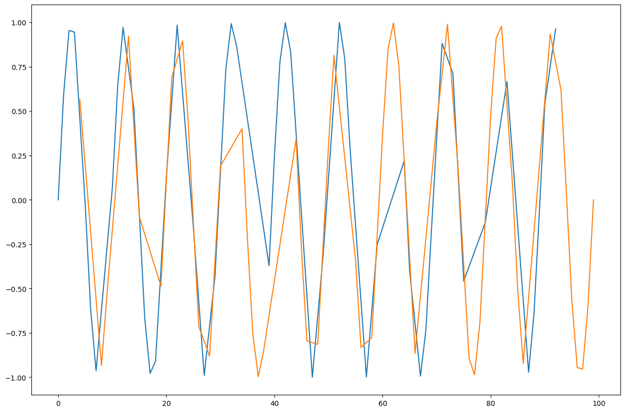
Plot the values of the grouped dataframe.
Solution
import matplotlib.pyplot as plt

fig, ax = plt.subplots(figsize=(15, 10))
grouped_plot = grouped.value.plot(ax=ax)
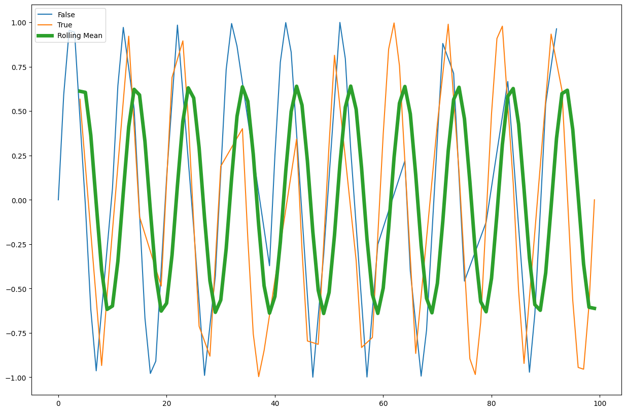
Use the
rolling()method to create a rolling average window of length 5 and overlay the result.
Solution
window_size = 5
rolling_mean = df.value.rolling(window=window_size).mean()
rolling_mean.plot(ax=ax, label="Rolling Mean", linewidth=5)
ax.legend(loc="upper left")
Other Pandas Features#
Pandas has a TON of features and small implementation details that are there to make your life simpler. Features like IntervalIndex to index the data between two numbers instead of having a single label, for example, are very nice and ergonomic if you need them. Sparse DataFrames are also included, as well as many other computational tools, serialization capabilities, and more. If you need it - there’s a good chance it already exists as a method in the pandas jungle.